Atomicity, Consistency, Isolation, and Durability are the four critical and fundamental properties that ensure reliable processing of database transactions.
Transaction
A collection of queries treated as a single unit of work.
Ensures that either all operations within the work unit are completed successfully or none are.
Example: Account Transfer (SELECT, UPDATE, UPDATE)
BEGIN;-- Debit ₹100 from account 1UPDATE accountsSET balance = balance - 100WHERE id = 1;-- Credit ₹100 to account 2UPDATE accountsSET balance = balance + 100WHERE id = 2;-- Commit if everything is fineCOMMIT;
Transaction Lifespan
BEGIN – Starts the transaction.
COMMIT – Finalizes all operations; changes become permanent.
ROLLBACK – Undoes all changes made by the transaction.
If a transaction ends unexpectedly (e.g., crash), ROLLBACK is automatically triggered.
Nature of Transactions
Primarily used to change and modify data.
Read-only transactions are also valid (e.g., generating consistent reports based on a snapshot).
Atomicity
Ensures that all operations in a transaction are completed successfully.
If any query fails, all prior successful operations within the same transaction are rolled back.
If the database crashes before COMMIT, all changes are undone.
Importance
Prevents partial updates.
Without atomicity, the database may be left in an inconsistent state.
Example
BEGIN;-- Debit ₹100 from account 1UPDATE accountsSET balance = balance - 100WHERE id = 1;-- Server crashes before the next update-- Credit ₹100 to account 2UPDATE accountsSET balance = balance + 100WHERE id = 2;-- COMMIT;
After reboot, account 1 is debited, but account 2 is not credited – Inconsistent data.
An atomic transaction would rollback the debit operation automatically.
Isolation
Ensures that concurrent execution of transactions results in a system state that would be obtained if the transactions were executed serially.
Read Phenomena
Dirty Read
Occurs when a transaction reads data that another transaction has written but not committed.
If the other transaction rolls back, the read data was invalid.
sequenceDiagram
    participant T1 as Transaction 1
    participant DB as Sales Table
    participant T2 as Transaction 2

    Note over DB: Initial State:<br/>id=1: price=100, quantity=2<br/>id=2: price=50, quantity=3

    T1->>DB: SELECT price*quantity FROM sales
    Note over DB: Returns total: 350

    T2->>DB: UPDATE sales SET price=120 WHERE id=1

    T1->>DB: SELECT SUM(price*quantity) FROM sales
    Note over DB: Returns incorrect total: 390

    T2-->>DB: ROLLBACK
    Note over DB: Reverts price to 100<br/>Final total should be 350
Non-repeatable Reads
Occur when a transaction reads the same row twice and gets different data due to modifications by another committed transaction.
Postgres (MVCC) never updates in place: an UPDATE writes a new row version (tuple); nothing is merged back. Old versions stay visible to older snapshots until VACUUM reclaims them.
MySQL InnoDB updates the row in place and keeps the old version in the undo log, which older snapshots (and ROLLBACK) use.
Phantom Read
Occurs when re-executing a query returns a different set of rows due to another committed transaction adding/removing rows.
Lost Update
Happens when two transactions read the same data and then update it, causing one update to overwrite the other.
Isolation Level
Dirty Read
Lost Updates
Non-repeatable
Phantom
Read Uncommitted
may occur
may occur
may occur
may occur
Read Committed
no
may occur
may occur
may occur
Repeatable Read
no
no
no
may occur
Serializable
no
no
no
no
Engine caveats: The table is the SQL-standard / lock-based view. Postgres RR (snapshot isolation) prevents phantoms too, and prevents lost updates by aborting the second writer with a serialization error. InnoDB RR still allows lost updates when you read-modify-write with a plain SELECT (use SELECT ... FOR UPDATE or an atomic UPDATE ... SET x = x + 1).
Database Isolation Implementations
Pessimistic: Uses locks (row/table/page) to avoid concurrency issues.
Optimistic: No locks; tracks data version and fails if conflicts arise.
Repeatable read “locks” the rows it reads but it could be expensive if you read a lot of rows, postgres implements RR as snapshot. That is why you don’t get phantom reads with postgres in repeatable read.
PostgreSQL uses snapshot isolation to implement Repeatable Read.
Serializable can be implemented optimistically (Postgres uses SSI – Serializable Snapshot Isolation – and aborts one transaction with a serialization error on conflict) or pessimistically with strict 2PL plus range/next-key locks (lock-based engines, e.g. InnoDB SERIALIZABLE). SELECT ... FOR UPDATE only locks the rows it returns; it is a manual tool, not how Serializable is implemented.
Consistency
Ensures that a transaction takes the database from one valid state to another valid state, preserving database invariants such as constraints and rules.
Consistency in Data
Defined by the schema, constraints, triggers, etc.
The LIKE count in the Pictures table matches the number of rows in Picture_Likes – data is consistent.
Consistency in Reads
Not ACID’s C: ACID consistency = invariants/constraints hold (the section above). Read consistency is a replication/distributed-systems property (CAP’s C = linearizable reads across nodes); they are different things.
Determines whether the result of a read reflects the most recent commit.
Crucial for distributed databases and replicas.
Eventual Consistency:
Guarantees the system will become consistent over time.
Categories:
Eventual Strong Consistency
Eventual Weak Consistency
Durability
Ensures that once a transaction is committed, its changes are permanent—even in case of system crash.
Durability Techniques
WAL (Write-Ahead Log):
Changes are logged before being written to disk.
Ensures recovery by replaying the log.
Append-Only Files (AOF):
Changes are appended to a file and replayed for recovery.
Asynchronous Snapshots:
Data held in memory is periodically persisted in batch.
OS-Level Durability
Writes go to OS cache before disk.
If system crashes before flushing cache, data is lost.
Use fsync to force flushing cache to disk for guaranteed durability.
How Tables and Indexes Are Stored on Disk and How They Are Queried
Storage Concepts
Table
Row ID
Page
IO
Heap data structure
Index data structure (B-tree)
Example of a query
Row ID
The Row ID is an internal and system-maintained identifier.
In some databases like MySQL (InnoDB), it is the same as the primary key.
In other databases like PostgreSQL, there is no row_id; the system column is ctid (the tuple ID: (page number, item index) of the row version in the heap). It changes when the row is updated or the table is rewritten, so it is not a stable identifier.
Page
Depending on the storage model (row store vs. column store), rows are stored and read in logical pages.
A database does not read a single row; it reads a page or more in a single IO operation.
Each page has a fixed size:
PostgreSQL: 8 KB
MySQL: 16 KB
For example, if each page holds 3 rows and you have 1001 rows, you’ll need approximately 1001 / 3 = 334 pages.
IO (Input/Output)
An IO operation is a read request to the disk.
IOs are expensive, so we try to minimize them.
An IO typically fetches an entire page (or more), not just a single row.
You get all the rows in the page “for free” once the page is loaded.
Some IOs can be served from the OS cache instead of accessing the physical disk.
Heap
A heap is a data structure where a table is stored with all its pages laid out sequentially.
This is where the actual data is stored — including all columns and rows.
Heap scans are expensive because you must read many pages to find what you need.
This is why indexes are used — they help pinpoint the exact page(s) you need to access in the heap.
Index
An index is a separate data structure from the heap and contains pointers to data in the heap.
It contains part of the data and is used to quickly locate rows.
You can index on one or more columns.
After locating a match in the index, the database follows a pointer to the heap to retrieve the full row.
An index helps avoid scanning the entire heap by telling you exactly which page to fetch.
Indexes are also stored in pages and thus require IO to access.
The smaller the index, the more likely it fits in memory, which results in faster searches.
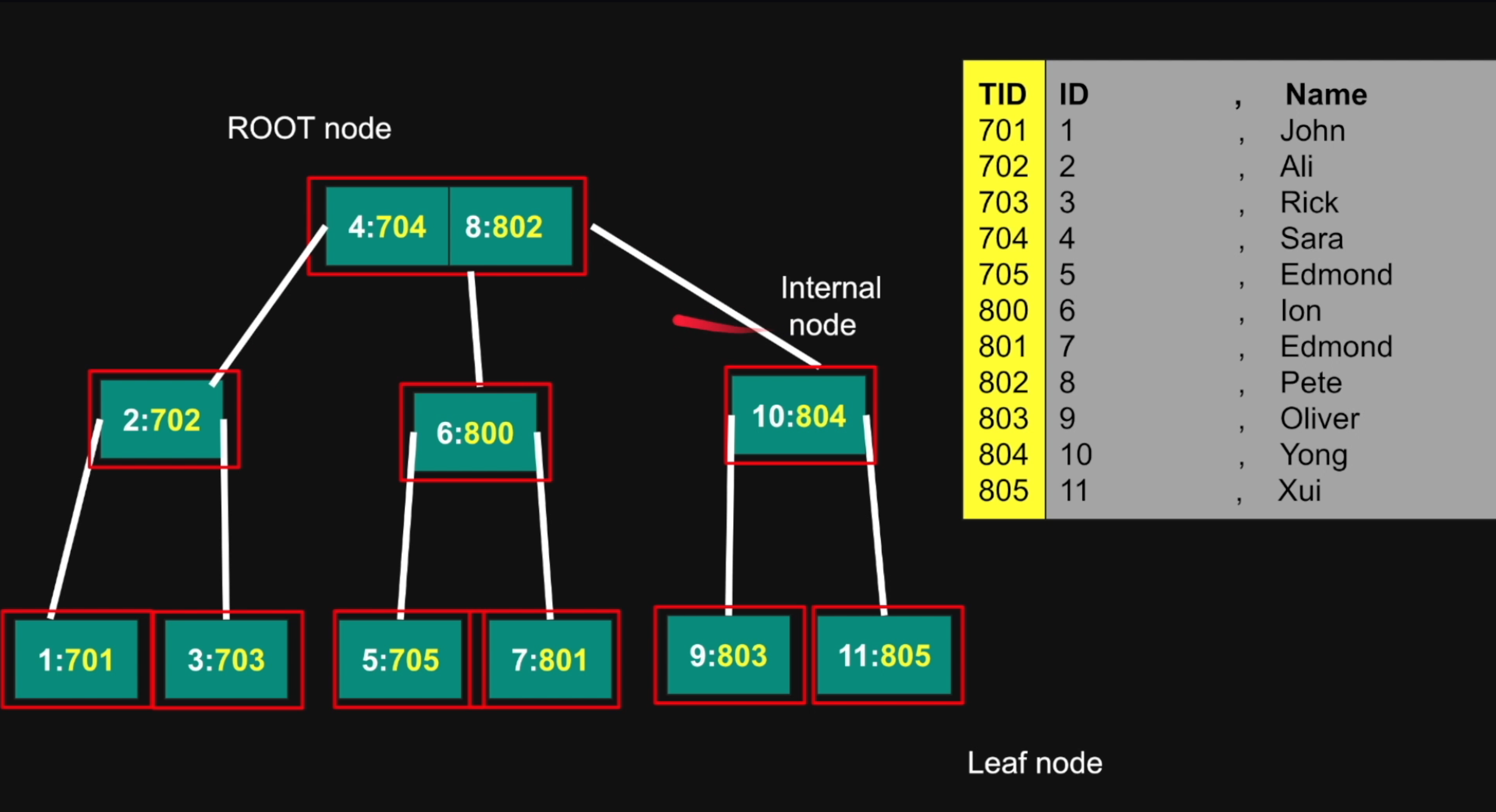
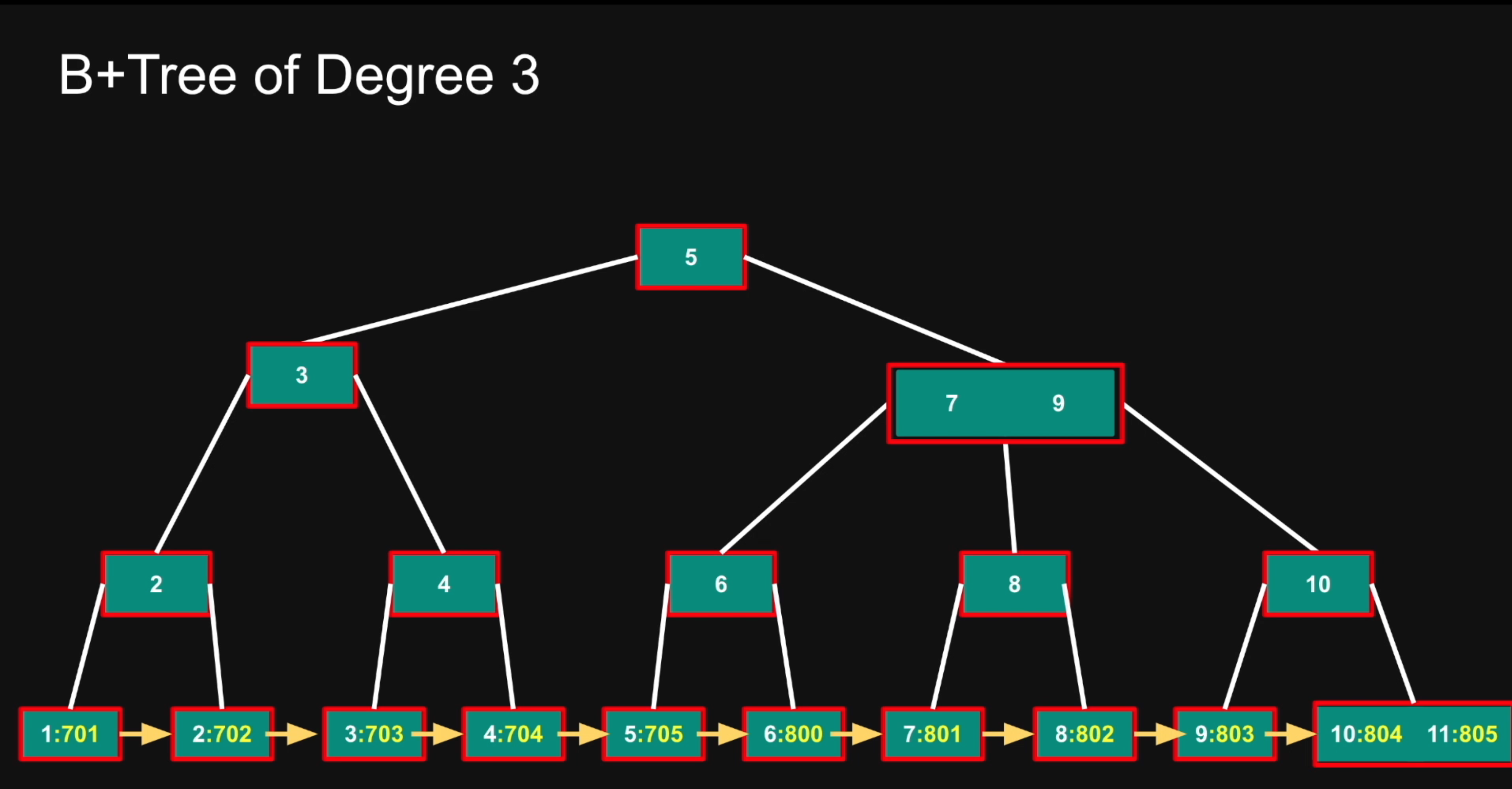
A common data structure for indexes is the B-tree.
Additional Notes
Sometimes the heap can be organized around a single index. This is called a clustered index or an Index Organized Table.
Whether the primary key is a clustered index depends on the engine: yes in InnoDB (and the SQL Server default); in PostgreSQL a PK is just a unique B-tree pointing into the unordered heap.
In MySQL (InnoDB):
There is always a primary key (clustered index).
Other indexes point to the primary key value.
In PostgreSQL:
All indexes are secondary indexes.
Indexes point directly to the row ID (ctid), which is located in the heap.
Indexing is a crucial technique used in databases to optimize data retrieval operations.
It improves query performance by minimizing disk I/O operations, thus reducing the time it takes to locate and access data.
Essentially, indexing allows the database management system (DBMS) to locate data more efficiently without having to scan the entire dataset.
Indexes are organized data structures that allow quick searching based on key values.
When an index is created for a database table, it maintains a sorted order of key values along with pointers to the actual data rows.
This process significantly reduces the number of disk accesses required to fulfill a query.
Create a index on table
Load 1 Million random data
--employees table for the indexing lecture--paste these commands into the postgres --start the docker instancedocker run --name pg -e POSTGRES_PASSWORD=postgres -d postgresdocker start pg--run postgres command shelldocker exec -it pg psql -U postgres--the command should switch to --postgres=#-- paste these sqlcreate table employees( id serial primary key, name text);create or replace function random_string(length integer) returns text as$$declare chars text[] := '{0,1,2,3,4,5,6,7,8,9,A,B,C,D,E,F,G,H,I,J,K,L,M,N,O,P,Q,R,S,T,U,V,W,X,Y,Z,a,b,c,d,e,f,g,h,i,j,k,l,m,n,o,p,q,r,s,t,u,v,w,x,y,z}'; result text := ''; i integer := 0; length2 integer := (select trunc(random() * length + 1));begin if length2 < 0 then raise exception 'Given length cannot be less than 0'; end if; for i in 1..length2 loop result := result || chars[1+random()*(array_length(chars, 1)-1)]; end loop; return result;end;$$ language plpgsql;insert into employees(name)(select random_string(10) from generate_series(0, 1000000));
create index employees_name on employees(name);
When getting id, name it will not search using the index employees_name.
LIKEcan use a B-tree index, but only when the pattern is a constant anchored at the start ('abc%') — Postgres turns it into a range scan (>= 'abc' AND < 'abd')
Leading wildcard ('%abc%', '%abc'): a B-tree can’t help → Seq Scan. Use a pg_trgm GIN index instead
Locale Gotcha: In a non-C locale (e.g. en_US.UTF-8, the usual default), a default index is not used even for 'abc%'. Create it with text_pattern_ops or COLLATE "C"
text_pattern_ops Trade-off: Serves LIKE 'abc%' and =, but not<, >, ORDER BY — keep a normal index too if you need those
ILIKE: B-tree only if the pattern starts with non-letters. Otherwise use pg_trgm
-- prefix search in a non-C localecreate index employees_name_pattern on employees(name text_pattern_ops);-- or: create index employees_name_c on employees(name collate "C");-- contains / ILIKE searchcreate extension pg_trgm;create index employees_name_trgm on employees using gin (name gin_trgm_ops);
In databases, clustering refers to how the physical storage of rows in a table is organized on disk based on a specific index—usually the primary key or another indexed column.
Clustered Index
A clustered index is an index that determines the physical order of data in a table.
There is only one clustered index per table because rows can only be stored in one physical order.
The table data itself is stored in the order of the clustered index.
In most relational databases:
MySQL (InnoDB): The primary key is always the clustered index (no PK → first UNIQUE NOT NULL index → else a hidden row id). You can’t cluster on any other column.
SQL Server: Lets you choose any clustered key (defaults to the PK).
PostgreSQL: Tables are heaps and are never truly clustered. CLUSTER is a one-off rewrite under an ACCESS EXCLUSIVE lock; the order isn’t maintained for new or updated rows.
CLUSTER table_name USING index_name;
Example
Consider a table of employees:
emp_id (PK)
name
salary
101
Alice
90,000
102
Bob
70,000
103
Carol
85,000
If emp_id is the clustered index:
The rows are stored physically ordered by emp_id.
If we create a clustered index on salary (possible in SQL Server; not in InnoDB, where only the PK clusters; in Postgres only as a one-off CLUSTER):
The table is reorganized so that rows are stored in order of salary.
Benefits of Clustering
Faster range queries: If you query a range of values (e.g., salary > 80,000), the database reads contiguous pages on disk.
Fewer I/O operations: Because related rows are stored together, fewer disk reads are needed.
Efficient sorting: Since data is already sorted physically, queries with ORDER BY can avoid extra sorting steps.
Drawbacks of Clustering
Slower inserts and updates: Because the DB must maintain the order, inserting a new row may require shifting other rows.
Only one per table: You can only cluster on one key.
Difference Between Clustered and Non-Clustered Index
Feature
Clustered Index
Non-Clustered Index
Physical order
Determines physical order of data
Does not affect physical row order
Number per table
Only one
Multiple allowed
Storage
Table and index are stored together
Index and table stored separately
Access
Faster for range queries
Requires additional lookup (to get full row)
Summary
Clustering in databases is the physical organization of data based on a particular key (usually via a clustered index), which helps in improving query performance—especially for range scans and ordered queries.
Purpose: Explore PostgreSQL’s specific implementation and design choices
Page Header (24 bytes)
Purpose: Fixed header containing page metadata
Content:
Information about page contents
Available free space tracking
Essential page management data
ItemIds (4 bytes each)
Function: Array of item pointers (not actual items/tuples)
Structure: Each ItemId = 4-byte offset:length pointer
Points To: Offset location and size of items within the page
HOT Optimization:
Enables Heap Only Tuple optimization
During updates, pointer redirects to new tuple location
Allows indexes to maintain references to old tuple ID
Very powerful for performance
Criticism:
At 4 bytes each, storage overhead can be significant
Example: an 8KB heap page holds at most ~291 tuples (MaxHeapTuplesPerPage) = ~1.2KB of line pointers; with small rows that’s still a big share of the page
Items (Variable length)
Content: Actual items/tuples stored sequentially
Layout: Items packed one after another
Terminology:
Row: What user sees
Tuple: Physical instance of row in page
Item: The tuple itself
MVCC Impact: Same row can have multiple tuples (active + historical + dead)
Special Section (Variable length)
Purpose: Index access-method-specific data
Applies To: Every page of every index type (B-tree, hash, GiST, GIN, SP-GiST, BRIN); for B-tree that means all pages (internal and leaf, plus the meta page). It is empty (size 0) on heap/table pages
Content: For B-tree, sibling links (previous/next page), the tree level and flags (leaf, root, deleted, etc.)
Function: Enables efficient B-tree traversal (e.g. range scans along the sibling links)
Tuple Referencing Example
Structure: Shows how tuples are referenced through ItemIds
Benefits: Indirection allows for optimizations like HOT
Summary
Key Concepts
Universal Storage: All database data ultimately stored in pages (indexes, sequences, tables)
Abstraction: Pages allow database to work uniformly regardless of content type
Structure: Pages contain headers and data, stored as files on disk
Flexibility: Each database implements different page layouts and storage methods
Common Principle: Consistent concept across all database systems despite implementation differences
Implementation Variations
Page Layout: Different databases use different internal page structures
Storage Methods: Various approaches to storing pages on disk
Optimization: Each system optimizes for different use cases and workloads
Standards: While concepts are universal, specific implementations vary significantly
Purpose: The primary goal of a query planner and optimizer is to find the most efficient way to execute a given SQL query. “Efficient” typically means minimizing resource consumption (CPU, I/O, memory) and therefore reducing query execution time.
Process Overview:
Parsing: The SQL query is parsed to check for syntactical correctness and to transform it into an internal representation (often a parse tree).
Binding/Validation: The objects referenced in the query (tables, columns, functions) are checked for existence and permissions. Data types are resolved.
Optimization (The Core): This is where the “magic” happens. The optimizer generates multiple possible execution plans for the query.
Logical Optimization: The query might be rewritten into an equivalent but potentially more efficient form using relational algebra rules (e.g., pushing predicates down, reordering joins).
Physical Optimization: For each logical plan, different physical operators are considered (e.g., hash join vs. nested loop join, full table scan vs. index scan).
Cost Estimation: Each potential execution plan is assigned a cost. This cost is an estimate based on:
Database Statistics: Information about the data distribution in tables and indexes (e.g., number of rows, distinct values, histograms). Keeping these statistics up-to-date is crucial for good performance.
Cost Model: A mathematical model that estimates the I/O, CPU, and other resource costs for different operations.
Plan Selection: The optimizer chooses the plan with the lowest estimated cost.
Execution: The chosen plan is then executed by the database engine.
Key Considerations in Optimization
Join Order: For queries involving multiple tables, the order in which tables are joined can dramatically impact performance. Optimizers spend significant effort evaluating different join orders.
Access Paths: How data is retrieved from tables:
Full Table Scan (Sequential Scan): Reads every row in the table. Efficient for small tables or when a large percentage of rows are needed.
Index Scan: Uses an index to directly locate specific rows. Much faster if the index is selective (i.e., it narrows down the search significantly).
Types of Index Scans: Unique scan, range scan, bitmap index scan (PostgreSQL).
Join Algorithms:
* Nested Loop Join: For each row in the outer table, scan the inner table. Good for small outer tables or when the inner table can be efficiently accessed via an index.
* Hash Join: Builds a hash table on one table (usually the smaller one) and then probes it with rows from the other table. Efficient for large tables and equi-joins.
* Merge Join: Requires both inputs to be sorted on the join columns. Then, it merges the sorted inputs. Efficient if inputs are already sorted or can be sorted cheaply.
Predicate Pushdown: Moving filtering conditions (WHERE clauses) as early as possible in the execution plan to reduce the amount of data processed by subsequent operations.
Subquery Handling: Optimizers have various strategies for handling subqueries, such as unnesting (converting them into joins), materializing them, or executing them as independent operations.
PostgreSQL Specifics
Genetic Query Optimizer (GEQO): For complex queries with many joins, PostgreSQL might use GEQO. This is a randomized algorithm that explores a subset of possible plans to find a good (though not necessarily the absolute best) plan in a reasonable amount of time. This is controlled by the geqo and geqo_threshold configuration parameters.
Cost Parameters: PostgreSQL has many configuration parameters (e.g., seq_page_cost, random_page_cost, cpu_tuple_cost) that influence the cost model. Tuning these (carefully!) can sometimes improve plan choices for specific workloads, but the defaults are generally well-tuned.
EXPLAIN Command: This is an indispensable tool in PostgreSQL (and most SQL databases).
EXPLAIN <QUERY>: Shows the optimizer’s chosen execution plan, including estimated costs, join methods, and access paths.
EXPLAIN ANALYZE <QUERY>: Executes the query and then shows the actual execution plan along with actual run times and row counts for each step. This is crucial for identifying performance bottlenecks and understanding if the optimizer’s estimates were accurate.
Statistics Collection: PostgreSQL’s ANALYZE command collects statistics about table data. Regular execution of ANALYZE (or autovacuum doing it automatically) is vital for the optimizer to make informed decisions.
VACUUM Command:
Purpose:VACUUM reclaims storage occupied by “dead tuples” (rows that have been deleted or made obsolete by an update). In PostgreSQL, updates and deletes don’t immediately remove old row versions; VACUUM is needed to clean them up and to prevent transaction ID wraparound.
VACUUM FULL: This is a more aggressive version that reclaims more space and can shrink the on-disk size of the table, but it takes an exclusive lock (blocking reads and writes) and can be very slow. It’s generally used infrequently and with caution.
VACUUM VERBOSE: Provides detailed output of the vacuuming process, showing which tables are being processed, the number of dead tuples removed, pages scanned, etc. For example, VACUUM VERBOSE students; would process the students table and show detailed logs.
VACUUM ANALYZE: This is a common and recommended practice. It first performs a VACUUM and then an ANALYZE on the specified table(s) or the entire database. For example, VACUUM ANALYZE students; or simply VACUUM ANALYZE;. This ensures that storage is reclaimed and statistics are updated in one operation.
Autovacuum: PostgreSQL has an autovacuum daemon that automates the execution of VACUUM and ANALYZE commands based on thresholds of table activity (inserts, updates, deletes). This is crucial for maintaining database performance, preventing table bloat, and ensuring fresh statistics without requiring constant manual intervention. While autovacuum handles most routine maintenance, manual VACUUM might be beneficial in specific scenarios (e.g., after very large bulk data modifications).
Impact on Query Planner: Regular vacuuming, especially when combined with ANALYZE (either manually or via autovacuum), ensures that the query planner has up-to-date statistics about data distribution. This leads to more accurate cost estimations, better query plan choices, and ultimately, improved query performance.
Planner Hints: While PostgreSQL generally discourages direct planner hints (unlike some other databases like Oracle), there are some extensions or ways to influence plans indirectly (e.g., by rewriting queries, creating specific indexes, or adjusting cost parameters). The philosophy is that the optimizer should be smart enough, and hints can become outdated or counterproductive as data or the database version changes.
Common Table Expressions (CTEs - WITH clauses): PostgreSQL’s optimizer can sometimes “inline” CTEs or materialize them. The MATERIALIZED and NOT MATERIALIZED keywords (PostgreSQL 12+) can give some control over this.
General SQL Optimizer Behavior
Rule-Based vs. Cost-Based Optimizers (RBO vs. CBO):
RBO: Uses a fixed set of rules and heuristics to choose a plan. Simpler but less flexible and often suboptimal. Largely historical, though some simple databases might still use aspects of it.
CBO: Uses a cost model and data statistics to estimate the cost of different plans and chooses the cheapest one. This is the standard in modern relational databases like PostgreSQL, MySQL, SQL Server, Oracle, etc.
Dynamic Sampling/Optimization: Some advanced optimizers can adjust plans mid-execution or gather more statistics on-the-fly if initial estimates seem poor, though this is less common for standard OLTP queries.
Why Understanding the Optimizer is Important
Performance Tuning: Knowing how the optimizer works helps in writing more efficient queries and designing appropriate indexes.
Troubleshooting: When a query is slow, EXPLAIN (or its equivalent) is the first step to understand why and what the optimizer decided to do.
Schema Design: Indexing strategies are directly related to how the optimizer will choose to access data.
Note on Primary Key Data Types
Caution with INT for Primary Keys: While INT (typically a 32-bit integer) can be used for primary keys, it’s crucial to be aware of its limitations for tables that might grow very large. The statement “Never set PRIMARY KEY as INT” is a strong generalization; INT can be acceptable for tables with a guaranteed small number of rows.
The Risk of Exhaustion:
A standard signed 32-bit INT has a maximum value of 2,147,483,647. An unsigned 32-bit INT can go up to 4,294,967,295.
If a table uses an auto-incrementing INT primary key and experiences a high volume of inserts (e.g., billions of rows, or fewer rows but with non-sequential ID usage or many deletions leading to higher sequence values), the available ID range can be exhausted.
Once exhausted, the database cannot assign new primary keys, effectively preventing new row insertions and potentially causing application failures. This is what’s meant by “blow up the database” – critical operations fail.
Why “Beyond a Billion Rows” is a Concern:
While a billion rows is less than the ~2.1 billion limit of a signed INT, it signifies a scale where INT exhaustion becomes a plausible risk, especially if IDs are not perfectly sequential from 1 or if the table has high churn (many inserts and deletes).
The actual limit is the maximum value of the INT type, not strictly the row count.
Recommended Alternatives for Large Tables:
BIGINT: This is typically a 64-bit integer, offering a much larger range (up to ~9 quintillion), making it a safer choice for auto-incrementing primary keys in tables expected to have many rows. Most modern database systems default to or recommend BIGINT for sequences.
UUID (Universally Unique Identifier): UUIDs are 128-bit values that are globally unique. They avoid exhaustion issues and can be generated in a distributed manner. However, they are larger, can lead to index fragmentation, and might be less human-readable.
Example of Integer Limit Issues (Analogous):
While specific public company admissions of database failures solely due to INT primary key exhaustion at exactly “1 billion rows” are not readily available (companies often don’t detail such internal issues), the principle of integer limits causing problems is well-known.
A famous public example of an integer limit being hit was YouTube’s view counter for the “Gangnam Style” video. The counter exceeded the maximum value for a 32-bit signed integer (2,147,483,647 views), forcing YouTube to upgrade their counter to a 64-bit integer. While this wasn’t a primary key for a database table in the same sense, it vividly illustrates the problem of data types being outgrown by scale.
Many large-scale platforms (social networks, e-commerce sites) proactively use BIGINT or UUIDs for their primary keys to prevent such scalability bottlenecks. The choice is a fundamental part of robust database design for high-growth applications.
When a database executes a SQL query, it needs to retrieve data from tables. The method it uses to access this data significantly impacts query performance. Here are three common scan methods: Sequential Scan, Index Scan, and Bitmap Index Scan.
Example Scenario
Let’s use the following employees table and indexes for our examples (syntax is generally PostgreSQL-like):
CREATE TABLE employees ( id SERIAL PRIMARY KEY, name VARCHAR(100) NOT NULL, department VARCHAR(50), salary INT, hire_date DATE, is_active BOOLEAN DEFAULT TRUE, country VARCHAR(50));-- Create some indexesCREATE INDEX idx_employees_salary ON employees (salary);CREATE INDEX idx_employees_department ON employees (department);CREATE INDEX idx_employees_is_active ON employees (is_active);CREATE INDEX idx_employees_country ON employees (country);CREATE INDEX idx_employees_dept_salary ON employees (department, salary);-- Populate with some sample data (conceptual)-- Imagine millions of rows in this table for a realistic scenario.INSERT INTO employees (name, department, salary, hire_date, is_active, country) VALUES('Alice Smith', 'Engineering', 70000, '2020-01-15', TRUE, 'USA'),('Bob Johnson', 'Marketing', 65000, '2019-03-01', TRUE, 'Canada'),('Charlie Brown', 'Engineering', 90000, '2021-07-22', TRUE, 'USA'),('Diana Prince', 'HR', 50000, '2018-05-10', FALSE, 'UK'),('Edward Nygma', 'Finance', 120000, '2017-11-01', TRUE, 'USA');-- ... and many more rows
1. Sequential Scan (Full Table Scan)
Explanation
A Sequential Scan reads every single row from the table, one by one, from the beginning to the end. It then evaluates each row against the conditions in the WHERE clause of the query.
When It’s Used
No Suitable Index: If there are no indexes on the columns used in the WHERE clause, or if the existing indexes cannot be effectively used for the given query conditions (e.g., using a function on an indexed column without a functional index).
Small Tables: For very small tables, the overhead of reading the entire table sequentially can be less than the overhead of using an index (which involves reading parts of the index and then potentially random access to table rows).
Low Selectivity / High Percentage of Rows: When the query is expected to retrieve a large percentage of the table’s rows. In such cases, reading all data blocks sequentially can be more efficient than performing many random I/O operations that an index scan might incur for a large number of rows. The database optimizer estimates the cost, and if most rows match, a sequential scan is cheaper.
COUNT(*) without a WHERE clause: Often, SELECT COUNT(*) FROM table; will result in a sequential scan if there isn’t a very small, covering index.
Pros
Simple and straightforward.
Efficient for small tables.
Can be efficient if a large portion of the table needs to be accessed.
Cons
Very inefficient for large tables if only a small number of rows are needed.
Can lead to high I/O and CPU usage for large tables.
Query Example for Sequential Scan
-- Querying on a non-indexed column or a condition that matches many rowsSELECT name, salaryFROM employeesWHERE hire_date > '2022-01-01';
Reasoning: If hire_date is not indexed, or if a very large number of employees were hired after this date, the database might opt for a sequential scan. Similarly, a query like SELECT * FROM employees WHERE name LIKE '%son%'; (leading wildcard) would also likely result in a sequential scan as standard B-tree indexes can’t efficiently handle leading wildcards.
2. Index Scan (or Index Seek / Range Scan)
Explanation
An Index Scan uses an index to locate specific rows in a table. The database traverses the index structure (commonly a B-tree) to find entries that match the query conditions. These index entries contain pointers (e.g., Row IDs or CTIDs in PostgreSQL) to the actual data rows in the table heap. The database then uses these pointers to fetch the required rows.
Index-Only Scan: A special, more efficient type of index scan occurs if all the columns requested by the query are present within the index itself. In this case, the database can skip the table heap for pages marked all-visible in the visibility map (set by VACUUM), saving I/O. The index doesn’t store MVCC visibility, so for other pages Postgres still checks the heap; on a frequently updated table Heap Fetches in EXPLAIN ANALYZE can be high.
When It’s Used
High Selectivity: When the query conditions are highly selective, meaning they retrieve a small number of rows relative to the table size.
Indexed Columns in WHERE Clause: The WHERE clause contains conditions on columns that have suitable indexes.
Equality and Range Predicates: For conditions like column = value, column > value, column BETWEEN value1 AND value2, column IN (val1, val2), or column LIKE 'prefix%' on indexed columns.
ORDER BY on an Indexed Column: If the query orders results by an indexed column, an index scan can retrieve rows in the sorted order, avoiding a separate sort step.
Pros
Very fast for retrieving a small number of rows from a large table.
Can avoid sorting if the index order matches the ORDER BY clause.
Index-only scans are extremely efficient.
Cons
“Tipping Point”: If the index scan needs to retrieve a large number of rows (low selectivity), it can become less efficient than a sequential scan. This is because it might involve many random I/O operations to fetch data from the table heap for each indexed row, which can be slower than sequentially reading all blocks.
Requires suitable indexes to be created and maintained (which adds overhead to write operations like INSERT, UPDATE, DELETE).
Index structure itself consumes disk space.
Query Example for Index Scan
-- Querying with a highly selective condition on an indexed columnSELECT id, name, departmentFROM employeesWHERE salary = 120000;
Reasoning: The salary column has an index (idx_employees_salary). If only a few employees have a salary of 120000, the optimizer will likely use an index scan on idx_employees_salary to quickly find these employees and then fetch their id, name, and department from the table.
-- Index-only scan example (if supported and applicable)SELECT department, salaryFROM employeesWHERE department = 'Engineering' AND salary > 80000;
Reasoning: The idx_employees_dept_salary covers both department and salary. If the database can satisfy the query by only reading this index (without going to the main table), it will perform an index-only scan.
3. Bitmap Index Scan (and Bitmap Heap Scan)
Explanation
The Bitmap Scan approach typically involves a sequence of operations, often seen in PostgreSQL execution plans. Let’s break down the key components:
Bitmap Index Scan:
* This is the initial step where the database scans a specific index (e.g., idx_employees_department for department = 'Engineering').
* Instead of fetching the table rows directly (like a regular Index Scan would for each found entry), it generates a bitmap in memory.
* This bitmap is a data structure that indicates which table pages (or sometimes individual rows, depending on granularity) contain rows matching the index condition. A bit is set for each page/row that qualifies.
* Multiple Bitmap Index Scans can be performed if there are multiple conditions on different indexes. For example, one for department = 'Engineering' and another for country = 'USA'.
BitmapAnd Scan / BitmapOr Scan:
* If multiple Bitmap Index Scans were performed (because of multiple AND or OR conditions on different indexes), the resulting bitmaps need to be combined.
* A BitmapAnd Scan takes two or more bitmaps and performs a bitwise AND operation on them. The resulting bitmap will only have bits set for pages/rows that were marked in all the input bitmaps. This is used for AND conditions (e.g., department = 'Engineering' AND country = 'USA').
* A BitmapOr Scan takes two or more bitmaps and performs a bitwise OR operation. The resulting bitmap will have bits set for pages/rows that were marked in any of the input bitmaps. This is used for OR conditions (e.g., department = 'Marketing' OR salary > 100000).
* These operations are very efficient as they work on compact bitmap structures in memory.
Bitmap Heap Scan:
* This is the final step where the actual data rows are retrieved from the table (the “heap”).
* It uses the final, combined bitmap (produced by one or more Bitmap Index Scans, possibly followed by BitmapAnd/BitmapOr operations).
* The database iterates through the table pages. If a page is marked in the final bitmap, that page is read from disk (if not already in memory).
* The rows within that page are then checked against the original query conditions to retrieve only the relevant ones.
* A key advantage is that pages are read from the table heap in physical order (or close to it), which can be more efficient than the potentially random I/O pattern of fetching individual rows scattered across the table, especially when a moderate number of rows are being retrieved.
In summary, the process often looks like this:
One or more Bitmap Index Scans create initial bitmaps.
If multiple bitmaps exist, they are combined using BitmapAnd Scan or BitmapOr Scan.
The resulting bitmap is used by a Bitmap Heap Scan to fetch the actual rows.
When It’s Used
Multiple Conditions on Different Indexed Columns: When a query has multiple conditions in the WHERE clause connected by AND or OR, and these conditions apply to different indexed columns.
Moderately Selective Conditions: When individual index conditions are not highly selective (i.e., they match a moderate number of rows), but their combination (using AND) becomes more selective.
OR Conditions on Different Indexes: Bitmap scans are particularly good at handling OR conditions across different indexes.
Low Cardinality Columns: For columns with a small number of distinct values (low cardinality) where a standard B-tree index scan might still retrieve many row pointers scattered across the table.
When the optimizer estimates that fetching rows in table-page order (guided by the bitmap) is more efficient than many random accesses from standard index scans.
Pros
Efficiently combines results from multiple indexes using bitwise operations on bitmaps.
Good for queries with AND/OR predicates on different indexed columns.
Can convert many random I/O operations into more sequential I/O for table access, improving performance for moderately selective queries.
Cons
Overhead: There’s an overhead in creating the bitmap(s). If the number of matching rows is very small, a direct index scan might be faster.
Dense Bitmaps: If the bitmap is very “dense” (meaning a very large percentage of rows/pages match the conditions), a sequential scan might be chosen by the optimizer instead, as the benefit of the bitmap diminishes.
The bitmap itself consumes memory. Large bitmaps for very large tables can be an issue.
Query Example for Bitmap Index Scan
-- Querying with multiple conditions on different indexed columnsSELECT name, salary, department, countryFROM employeesWHERE department = 'Engineering' AND is_active = TRUE AND country = 'USA';
Reasoning:
Here, we have conditions on department (indexed by idx_employees_department), is_active (indexed by idx_employees_is_active), and country (indexed by idx_employees_country).
The database might perform:
A Bitmap Index Scan on idx_employees_department for department = 'Engineering' to create bitmap1.
A Bitmap Index Scan on idx_employees_is_active for is_active = TRUE to create bitmap2.
A Bitmap Index Scan on idx_employees_country for country = 'USA' to create bitmap3.
Combine these bitmaps using bitwise AND: final_bitmap = bitmap1 AND bitmap2 AND bitmap3.
Perform a Bitmap Heap Scan using final_bitmap to retrieve the matching rows from the employees table.
Another example with OR:
SELECT name, salary, departmentFROM employeesWHERE department = 'Marketing' OR salary > 100000;
Reasoning:
The database could create one bitmap for department = 'Marketing' (using idx_employees_department) and another for salary > 100000 (using idx_employees_salary), then combine them with a bitwise OR, followed by a Bitmap Heap Scan.
Note: The actual execution plan chosen by a database optimizer depends on many factors, including table statistics (size, data distribution, cardinality), index availability, query structure, and database configuration parameters. Using EXPLAIN (or EXPLAIN ANALYZE in PostgreSQL) is crucial for understanding how a specific query is being executed.
Database indexes are crucial for query performance. They can be broadly categorized based on whether they are built on “key” columns (which enforce uniqueness or serve as primary identifiers) or “non-key” columns (used for general query optimization).
Example Scenario
Let’s use the following products table for our examples:
CREATE TABLE products ( product_id INT PRIMARY KEY, -- Key column (Primary Key) product_sku VARCHAR(50) UNIQUE, -- Key column (Unique Key) product_name VARCHAR(255) NOT NULL, category_id INT, supplier_id INT, price DECIMAL(10, 2), is_active BOOLEAN DEFAULT TRUE, last_updated TIMESTAMP DEFAULT CURRENT_TIMESTAMP);-- Example of creating a non-key column indexCREATE INDEX idx_products_category_id ON products (category_id);-- Example of a composite non-key column indexCREATE INDEX idx_products_supplier_price ON products (supplier_id, price);-- Example of a non-key index that might be used for filtering and orderingCREATE INDEX idx_products_last_updated ON products (last_updated DESC);
1. Key Column Indexes
These are indexes built on columns that have a special role in identifying or constraining data in a table.
a. Primary Key Index
Definition: An index automatically created (in most RDBMS) when a PRIMARY KEY constraint is defined on a column or set of columns. The primary key uniquely identifies each row in the table.
Implicit Creation: You typically don’t create a primary key index manually; it’s part of defining the primary key constraint.
In our example: product_id INT PRIMARY KEY will automatically create a primary key index on product_id.
Characteristics:
Uniqueness: Enforces that all values in the primary key column(s) are unique.
Row Identification: Serves as the main way to uniquely identify and access a specific row.
Clustering (System Dependent):
In some RDBMS like SQL Server, the primary key index is, by default, a clustered index. This means the physical order of data rows in the table is the same as the order of the primary key index. A table can have only one clustered index.
In MySQL (InnoDB), the primary key index is the clustered index: its leaf pages store the full rows, i.e. the PK index is the table. Every other index is secondary and stores the PK value to find the row.
In PostgreSQL, all indexes (including the primary key index) are secondary indexes that point (via ctid) to rows in a separate heap table; there is no clustered PK.
Purpose:
Uniquely identify rows.
Enforce entity integrity.
Serve as the target for foreign key relationships from other tables.
Provide fast lookups when searching for a specific row by its primary key value (e.g., SELECT * FROM products WHERE product_id = 123;).
b. Unique Key Index
Definition: An index automatically created when a UNIQUE constraint is defined on a column or set of columns. This ensures that all values in the specified column(s) are unique across the table.
Implicit Creation: Similar to primary key indexes, these are usually created as part of the constraint definition.
In our example: product_sku VARCHAR(50) UNIQUE will automatically create a unique index on product_sku.
Characteristics:
Uniqueness: Enforces that all values in the indexed column(s) are unique.
Allows NULLs (Typically): Unlike primary keys, unique key columns can often allow NULL values (though the exact behavior with multiple NULLs can vary between RDBMS and how the constraint is defined).
Secondary Identifiers: Can serve as alternative ways to uniquely identify rows.
Purpose:
Enforce uniqueness on non-primary key columns.
Provide alternative unique identifiers for rows.
Enable fast lookups based on these unique values (e.g., SELECT * FROM products WHERE product_sku = 'ABC-12345';).
2. Non-Key Column Indexes (Secondary or Auxiliary Indexes)
These are indexes created on columns that are not necessarily unique and are not primary keys. Their main purpose is to improve query performance.
Definition: Indexes explicitly created by a user or DBA on one or more columns to speed up data retrieval operations, filtering (WHERE clause), sorting (ORDER BY clause), and join operations.
Explicit Creation: Created using the CREATE INDEX statement.
In our example: CREATE INDEX idx_products_category_id ON products (category_id); creates a non-key index on the category_id column.
CREATE INDEX idx_products_supplier_price ON products (supplier_id, price); creates a composite non-key index.
Characteristics:
No Uniqueness Enforcement (by default): These indexes do not inherently enforce uniqueness. The indexed columns can contain duplicate values.
Pointers to Data: A non-key index stores the indexed column value(s) and a pointer (e.g., RowID, CTID, or the primary key value if the table has a clustered primary key) to the actual data row in the table.
Always Non-Clustered (in the sense of table organization): They do not dictate the physical storage order of the table rows themselves (unlike a clustered primary key in some systems). They are separate structures.
Purpose:
Speed up WHERE clause filtering: Queries like SELECT * FROM products WHERE category_id = 10; can use idx_products_category_id to quickly find matching rows instead of scanning the entire table.
Improve JOIN performance: If category_id is used in a JOIN with another table, this index can make the join faster.
Optimize ORDER BY and GROUP BY: Queries like SELECT category_id, COUNT(*) FROM products GROUP BY category_id; or SELECT * FROM products ORDER BY last_updated DESC; can benefit from indexes on category_id and last_updated respectively, potentially avoiding costly sort operations.
Covering Indexes: A powerful type of non-key index. If an index contains all the columns requested by a query (both in the SELECT list and the WHERE clause), the database can answer the query by reading only the index, without accessing the table itself. This is called an index-only scan and is very efficient.
Example: For the query SELECT supplier_id, price FROM products WHERE supplier_id = 5;, the index idx_products_supplier_price could potentially be a covering index if the database optimizer chooses to use it this way.
Primary Key: Not allowed. Unique Key: Usually allowed.
Allowed (unless column constraint prevents it)
Creation
Often implicit with PRIMARY KEY or UNIQUE constraints
Explicit via CREATE INDEX statement
Table Clustered By
Primary Key often dictates clustering in some RDBMS
Typically non-clustered (separate from table data order)
Number Per Table
One Primary Key. Multiple Unique Keys.
Multiple non-key indexes allowed.
4. Considerations
Write Overhead: All indexes (key or non-key) add overhead to write operations (INSERT, UPDATE, DELETE). When data is modified, the corresponding indexes must also be updated. Too many indexes can slow down writes.
Storage Space: Indexes consume disk space.
Selectivity: Indexes are most effective on columns with high selectivity (many distinct values relative to the total number of rows). Indexes on low-selectivity columns (e.g., a boolean is_active column in a very large table where most values are TRUE) might not be used by the optimizer or could even be detrimental, though bitmap indexes can be useful here.
Query Patterns: Choose indexes based on the actual queries your application runs. Analyze slow queries to identify candidate columns for indexing.
Maintenance: Indexes may require maintenance (e.g., rebuilding or reorganizing) to remain efficient over time as data changes.
Understanding the distinction between key and non-key column indexes helps in designing efficient database schemas and optimizing query performance effectively.
In relational databases, ACID is a set of properties that ensure reliable and consistent transaction processing.
What is ACID?
Property
Description
Atomicity
Ensures that all operations in a transaction are completed or none are.
Consistency
Ensures the database transitions from one valid state to another.
Isolation
Ensures transactions are executed independently, avoiding interference.
Durability
Once committed, changes are permanent, even in case of system failure.
Example Setup
CREATE TABLE products ( pid serial primary key, name text, price float, inventory integer);CREATE TABLE sales ( saleid serial primary key, pid integer, price float, quantity integer);-- Insert initial productINSERT INTO products (name, price, inventory) VALUES('Phone', 999, 100);
Transaction Block Example
BEGIN TRANSACTION; SELECT * FROM products; -- Check current inventory UPDATE products SET inventory = inventory - 10; -- Reduce stock SELECT * FROM products; -- Confirm updated inventory INSERT INTO sales (pid, price, quantity) VALUES(1, 999, 10); -- Record saleCOMMIT;
Breakdown of ACID in This Example
Atomicity
The block of operations is treated as a single unit.
If any step (e.g., the INSERT INTO sales) fails, the entire transaction is rolled back, and no partial changes are saved.
Consistency
The transaction ensures that:
The inventory is correctly reduced by 10.
A corresponding entry is added to sales.
The database moves from one valid state (inventory: 100) to another valid state (inventory: 90 with matching sale record).
Isolation
BEGIN TRANSACTION ISOLATION LEVEL REPEATABLE READ;
This isolation level ensures that:
This transaction reads from a snapshot taken at its first query, so it never sees other transactions’ later commits.
Prevents issues like non-repeatable reads and (in Postgres) phantom reads.
Other transactions can still modify the rows this transaction read (plain reads take no row locks under MVCC).
A plain SELECT never waits for row locks at any isolation level, even inside BEGIN; it returns the last committed value. Only SELECT ... FOR SHARE/FOR UPDATE and UPDATE/DELETE of the same row wait for the other transaction to commit or roll back (DDL like ALTER TABLE/TRUNCATE blocks even plain SELECTs).
If this transaction later tries to update a row that another transaction changed and committed, Postgres aborts it with a serialization error (could not serialize access due to concurrent update); the application must retry.
Durability
Once COMMIT; is executed:
The changes to both products and sales are persisted permanently.
Even if the system crashes immediately afterward, the data remains intact in the database.
Summary
Property
Ensured By
Atomicity
BEGIN … COMMIT; - All or nothing
Consistency
Proper business logic and relational constraints
Isolation
ISOLATION LEVEL REPEATABLE READ or higher
Durability
Underlying database commit and logging system
This example illustrates how a single logical unit of work adheres to ACID principles to maintain data integrity and reliability.
A phantom read occurs when a transaction executes the same query multiple times and sees different results due to other transactions inserting or deleting rows that match the query’s WHERE clause.
Example Scenario:
Assume the sales table initially has:
amounts: 100, 200, 300
Transaction 1 (T1):
BEGIN;SELECT COUNT(*) FROM sales WHERE amount > 150; -- Returns 2
Meanwhile, Transaction 2 (T2):
BEGIN;INSERT INTO sales (amount) VALUES (250);COMMIT;
Back to T1:
BEGIN;SELECT COUNT(*) FROM sales WHERE amount > 150; -- Returns 3 (phantom row!)COMMIT;
T1 sees different results between two reads — a classic phantom read.
Visualization with Mermaid
Sequence Diagram
sequenceDiagram
    participant T1 as Transaction 1<br/>(Read Committed)
    participant DB as Database
    participant T2 as Transaction 2

    Note over T1,T2: Initial state: sales table contains<br/>amounts: 100, 200, 300

    T1->>DB: BEGIN
    T1->>DB: SELECT COUNT(*)<br/>FROM sales WHERE amount > 150
    DB-->>T1: Returns count: 2

    T2->>DB: BEGIN
    T2->>DB: INSERT INTO sales<br/>(amount) VALUES (250)
    T2->>DB: COMMIT

    T1->>DB: SELECT COUNT(*)<br/>FROM sales WHERE amount > 150
    DB-->>T1: Returns count: 3<br/><i>(Phantom row appears)</i>

    T1->>DB: COMMIT
Handling Phantom Reads in PostgreSQL
Isolation Levels Overview
flowchart LR
    subgraph "PostgreSQL Isolation Levels"
        RC["Read Committed<br/><i>(Default)</i>"] --> RR["Repeatable Read"] --> SER["Serializable"]

        RC --> RC_desc["• Allows phantom reads<br/>• Fastest performance<br/>• Good for simple reads"]
        RR --> RR_desc["• Prevents phantom reads<br/>• Strong consistency<br/>• May need retries"]
        SER --> SER_desc["• Maximum isolation<br/>• Full consistency<br/>• Highest overhead"]
    end

    style RC fill:#ffcccc,stroke:#ff9999,color:#000000
    style RR fill:#ffffcc,stroke:#ffcc99,color:#000000
    style SER fill:#ccffcc,stroke:#99ff99,color:#000000
PostgreSQL Implementation
Using Serializable Isolation (Prevents Phantom Reads)
-- Transaction 1BEGIN TRANSACTION ISOLATION LEVEL SERIALIZABLE;SELECT COUNT(*) FROM sales WHERE amount > 150; -- Returns 2-- Transaction 2 (in another session)BEGIN TRANSACTION ISOLATION LEVEL SERIALIZABLE;INSERT INTO sales (amount) VALUES (250);COMMIT;-- Back to Transaction 1SELECT COUNT(*) FROM sales WHERE amount > 150; -- Still returns 2 (reads its snapshot, no phantom)COMMIT; -- Both transactions commit: a read-only T1 doesn't conflict
Prevents phantom reads
T1 just keeps seeing its snapshot; no error here. A serialization error only happens when the concurrent transactions form a read/write dependency cycle (e.g. T1 also writes based on the count it read)
Highest consistency
May fail with serialization errors (needs retry)
Using Read Committed (Default)
-- Transaction 1BEGIN;SELECT COUNT(*) FROM sales WHERE amount > 150; -- Returns 2-- Transaction 2 (in another session)BEGIN;INSERT INTO sales (amount) VALUES (250);COMMIT;-- Back to Transaction 1SELECT COUNT(*) FROM sales WHERE amount > 150; -- Returns 3 (phantom read!)COMMIT;
Fast and simple
Allows phantom reads
Not ideal for critical operations
Preventing Phantom Reads in PostgreSQL
Use SERIALIZABLE isolation level
Use REPEATABLE READ (in Postgres it is snapshot isolation, so phantoms don’t appear)
Apply explicit locks
Example:
LOCK TABLE sales IN SHARE MODE; -- blocks concurrent INSERT/UPDATE/DELETE until commit
Note: SELECT ... FOR SHARE only locks the rows that already exist; Postgres has no gap/range locks, so it does not stop other transactions inserting new matching rows.
Implement application-level locking mechanisms
Trade-offs
Isolation Level
Phantom Read
Performance
Use Case
Read Committed
Yes
Fast
Simple reads, non-critical logic
Repeatable Read
No
Medium
Consistency-focused apps
Serializable
No
Slower
Mission-critical, consistent reads
Conclusion
Phantom reads are a significant concurrency issue in databases that affect consistency during concurrent transactions. Choosing the right isolation level and concurrency control mechanism is essential based on the application’s consistency and performance requirements.
NOTE
Postgres’s default level, Read Committed, allows phantom reads (see the example above). Postgres prevents them at Repeatable Read (snapshot) and Serializable (SSI) – stricter than the SQL standard, which only requires it at Serializable.
Definition:
Occurs when a transaction reads the same row twice and gets different values, because another transaction modified and committed the row between the two reads.
Example:
-- Transaction ABEGIN;SELECT balance FROM accounts WHERE id = 1; -- returns ₹1000-- Meanwhile, Transaction BBEGIN;UPDATE accounts SET balance = 1200 WHERE id = 1;COMMIT;-- Back to Transaction ASELECT balance FROM accounts WHERE id = 1; -- returns ₹1200 now
Issue: Transaction A saw two different values without making any changes.
Occurs in: Read Committed isolation level.
Prevented in: Repeatable Read and Serializable.
Serializable
Definition:
The highest isolation level. Ensures that transactions are executed in a serial order, i.e., one after the other — even if executed concurrently. It prevents all anomalies, including dirty reads, non-repeatable reads, and phantom reads.
Guarantee:
The outcome is as if transactions were executed one at a time, not concurrently.
How it prevents non-repeatable reads:
Lock-based engines (strict 2PL, e.g. InnoDB SERIALIZABLE with autocommit off, where plain SELECT becomes SELECT ... FOR SHARE): reads take shared locks, so concurrent writes to those rows wait.
MVCC engines (Postgres SSI): each transaction reads its snapshot, so re-reads return the same data. Other transactions can still modify the rows; if that creates a conflict that breaks serial order, one transaction is aborted with a serialization error (usually at commit) and must be retried.
In Postgres a plain SELECT never waits for row locks, even under SERIALIZABLE; it returns the last committed version. Only locking reads (FOR SHARE/FOR UPDATE) and UPDATE/DELETE of the same row wait.
Comparison Table
Feature
Non-Repeatable Read
Serializable
What it is
An anomaly / problem
An isolation level (solution)
Problem or Solution?
Problem
Solution
Prevents Dirty Read
❌ Not necessarily
✅ Yes
Prevents Non-repeatable Read
❌ No
✅ Yes
Prevents Phantom Read
❌ No
✅ Yes
Used In
Lower isolation levels (Read Committed)
Highest level of isolation
🧠 TL;DR
Non-repeatable read is a problem caused by another transaction changing data between two reads.
Serializable is an isolation level that prevents this and other issues by ensuring transactions behave as if run one by one.
Eventual Consistency is a consistency model used in distributed systems (like NoSQL databases) that guarantees that, if no new updates are made to a given piece of data, eventually all accesses to that data will return the same latest value.
It does not guarantee immediate consistency, but ensures that data will be consistent over time.
Real-Life Analogy
Imagine you’re updating your Instagram bio. Your profile shows the new bio instantly, but your friend on another continent might see the old bio for a few seconds due to server lag. After a short time, everyone sees the new bio — that’s eventual consistency.
Characteristics
Prioritizes availability and partition tolerance (CAP theorem).
High performance and scalability.
Updates may not be immediately visible to all nodes.
Eventually, all replicas converge to the same state.
An Index Scan is a method used by a database to retrieve data from a table by first looking up values in an index and then using those index entries to locate and retrieve the corresponding rows from the table itself.
Process:
The database traverses the index to find entries that match the query’s conditions.
For each matching index entry, the database obtains a pointer (e.g., a row ID or RID) to the actual row in the table.
The database uses this pointer to access the table heap and retrieve the required columns for that row.
When it’s used:
When the query needs to select columns that are not part of the index.
The index helps narrow down the rows to be fetched, but the table access is still necessary to get all the requested data.
Characteristics:
Involves two main I/O operations: one to read the index and another to read the table data.
Can be slower than an Index Only Scan if many rows need to be fetched from the table, as this involves random I/O to the table heap.
Index Only Scan
An Index Only Scan is a more efficient data retrieval method where the database can satisfy the entire query (i.e., retrieve all requested columns) directly from an index without accessing the table itself.
Process:
The database traverses the index to find entries that match the query’s conditions.
All the columns required by the query are present within the index itself.
The database retrieves the data directly from the index, skipping the table heap for pages marked all-visible.
PostgreSQL caveat: the index has no visibility (MVCC) info, so for each row the planner checks the visibility map; if the row’s heap page is not all-visible (recently modified, not yet VACUUMed) it still fetches the heap tuple (shown as Heap Fetches in EXPLAIN ANALYZE). Running VACUUM keeps the visibility map up to date.
When it’s used:
When all columns selected in the query are part of the index (e.g., in a covering index).
For queries like COUNT(*) where the index can provide the count without needing to access the table.
Characteristics:
Involves only one main I/O operation: reading the index.
Significantly faster than an Index Scan because it avoids most of the I/O cost of accessing the table heap (all of it only when the pages are all-visible).
Reduces I/O and can improve query performance, especially for queries that select a small number of columns that are all covered by an index.
Key Differences Summarized
Feature
Index Scan
Index Only Scan
Table Access
Yes, accesses table heap after index lookup.
Only for heap pages not all-visible in the visibility map (Postgres); otherwise none.
Columns
Can retrieve any column from the table.
Can only retrieve columns present in the index.
I/O Operations
Reads index + Reads table data.
Reads index (+ visibility map, + heap for non-all-visible pages).
Performance
Generally slower due to table access.
Generally faster as it avoids table access.
Use Case
Query selects columns not in the index.
All selected columns are in the index (covering index).
When to Optimize for Index Only Scans
Identify frequently executed queries that select a limited set of columns.
Consider creating covering indexes that include all the columns needed by these queries in the SELECT, WHERE, ORDER BY, and GROUP BY clauses.
Be mindful of the trade-offs: adding too many columns to an index can increase its size, potentially slowing down write operations (INSERT, UPDATE, DELETE) and consuming more storage.
Regularly analyze query performance and index usage to ensure that the indexes are still beneficial as the data and query patterns evolve.
Additional Notes on Non-Key Columns
Non-key columns (also known as included columns or non-key attributes) are columns that are part of a non-clustered index but are not part of the index key itself. Their primary purpose is to support Index Only Scans.
Benefits in the context of Index Scans vs. Index Only Scans:
Facilitating Index Only Scans:
By including non-key columns in an index, you can create “covering indexes.” If a query requests columns that are all present either as key columns or as included non-key columns in the index, the database can perform an Index Only Scan.
This avoids the need to access the table heap (as in a regular Index Scan), significantly improving query performance by reducing I/O.
Selectivity vs. Coverage:
Index Key Columns: These are used for searching and sorting data within the index. The selectivity of these columns (how many unique values they have) is crucial for the efficiency of index seeks.
Non-Key (Included) Columns: These are not used for searching or sorting within the index structure itself. They are simply stored at the leaf level of the index alongside the key values. Their presence allows the query to be “covered” by the index.
Impact on Index Size and Maintenance:
Adding non-key columns increases the overall size of the index. Larger indexes consume more disk space and can potentially slow down Data Manipulation Language (DML) operations (INSERT, UPDATE, DELETE) because the index also needs to be updated.
It’s a trade-off: you improve read performance for specific queries at the cost of storage and potentially write performance.
When to Use Included Columns:
When you have queries that frequently select specific columns that are not part of the primary search criteria (i.e., not ideal as key columns).
To avoid making the index key too wide. Wide index keys can reduce the effectiveness of the B-tree structure. Including columns as non-key attributes is often a better alternative than adding them to the index key if they are not used for filtering or sorting.
For columns with data types that are not suitable for index keys (e.g., large text or binary objects), though it’s generally better to avoid including very large columns even as non-key columns if possible.
Example Scenario:
Consider a table Employees with columns EmployeeID (PK), DepartmentID, Salary, HireDate, and Email.
An index on (DepartmentID) would lead to an Index Scan:
Index seek on DepartmentID.
For each match, a key lookup (RID lookup) into the Employees table to fetch the Email.
An index on (DepartmentID) with Email as an included non-key column (e.g., CREATE INDEX IX_Dept_Email ON Employees (DepartmentID) INCLUDE (Email);) would lead to an Index Only Scan:
Index seek on DepartmentID.
The Email is available directly from the leaf level of the index. No table access is needed.
By carefully choosing which non-key columns to include, you can significantly boost the performance of targeted queries by enabling Index Only Scans.
Database-Specific Examples
Example Table Schema
Let’s use the following example table schema for demonstrations:
CREATE TABLE products ( product_id INT PRIMARY KEY, category_id INT NOT NULL, product_name VARCHAR(100) NOT NULL, description TEXT, price DECIMAL(10,2) NOT NULL, stock_quantity INT NOT NULL, created_at TIMESTAMP DEFAULT CURRENT_TIMESTAMP);
PostgreSQL Examples
Creating Indexes in PostgreSQL
-- Create a regular index (will result in Index Scan for most queries)CREATE INDEX idx_category ON products(category_id);-- Create a covering index to enable Index Only ScansCREATE INDEX idx_category_covering ON products(category_id) INCLUDE (product_name, price);
Analyzing PostgreSQL Execution Plans
You can use the EXPLAIN ANALYZE command to see which type of scan PostgreSQL chooses:
-- This query will likely use an Index Scan because description is not in the indexEXPLAIN ANALYZESELECT product_name, description, priceFROM productsWHERE category_id = 5;-- This query can use an Index Only Scan because all selected columns are in the covering indexEXPLAIN ANALYZESELECT product_name, priceFROM productsWHERE category_id = 5;
Expected output showing an Index Only Scan:
Index Only Scan using idx_category_covering on products
  Index Cond: (category_id = 5)
  Heap Fetches: 0  -- No heap fetches: all pages were all-visible (a high number means VACUUM is needed)
Controlling PostgreSQL Scan Behavior
PostgreSQL allows you to control the query planner behavior:
-- Disable Index Only Scans to force Index ScansSET enable_indexonlyscan = off;EXPLAIN ANALYZESELECT product_name, priceFROM productsWHERE category_id = 5;-- Re-enable Index Only ScansSET enable_indexonlyscan = on;
MySQL Examples
Creating Indexes in MySQL
-- Create a regular index (will result in Index Scan for most queries)CREATE INDEX idx_category ON products(category_id);-- Create a covering index to enable Index Only Scan capabilitiesCREATE INDEX idx_category_name_price ON products(category_id, product_name, price);
Analyzing MySQL Execution Plans
In MySQL, you can use EXPLAIN to view the execution plan:
-- This query will likely use an Index Scan (ref in MySQL terminology)-- because it needs to access the table for the description columnEXPLAINSELECT product_name, description, priceFROM productsWHERE category_id = 5;-- This query can be satisfied using only the index (covering index)EXPLAINSELECT product_name, priceFROM productsWHERE category_id = 5;
Expected output for Index Only Scan in MySQL:
+----+-------------+----------+------------+------+---------------+-----------------------+---------+-------+------+----------+-------------+| id | select_type | table | partitions | type | possible_keys | key | key_len | ref | rows | filtered | Extra |+----+-------------+----------+------------+------+---------------+-----------------------+---------+-------+------+----------+-------------+| 1 | SIMPLE | products | NULL | ref | idx_category | idx_category_name_price | 4 | const | 10 | 100.00 | Using index |+----+-------------+----------+------------+------+---------------+-----------------------+---------+-------+------+----------+-------------+
The Using index in the Extra column indicates that MySQL can satisfy the query using only the index (an Index Only Scan).
Controlling MySQL Scan Behavior
MySQL allows some control over optimizer behavior:
-- Use index hints to force the use of a specific indexSELECT product_name, priceFROM products FORCE INDEX (idx_category_name_price)WHERE category_id = 5;-- Ignore an index to prevent its useSELECT product_name, priceFROM products IGNORE INDEX (idx_category_name_price)WHERE category_id = 5;
Performance Comparison
When working with large tables:
Index Scan: May require thousands of random I/O operations to fetch rows from the table, especially when retrieving many rows.
Index Only Scan: Might be 2-10 times faster depending on the scenario, as it avoids these random I/O operations by reading only from the index structure.
Understanding these scan methods and designing your indexes accordingly can dramatically improve the performance of your database queries in production environments.
A Normal Index (also called a single-column index) is created on a single column of a table. It speeds up queries that filter, sort, or join on that specific column.
CREATE INDEX idx_column_a ON table_name(column_a);
Composite (Multi-Column) Index
A Composite Index is created on two or more columns of a table. It can speed up queries that filter, sort, or join on any leading column(s) of the index.
CREATE INDEX idx_column_a_b ON table_name(column_a, column_b);
Query Performance Analysis
Let’s analyze different query scenarios using a table with columns a and b, and compare the performance impacts of different indexing strategies.
Example Table Schema
CREATE TABLE example_table ( id INT PRIMARY KEY, column_a INT, column_b VARCHAR(50), other_data TEXT);
Scenario 1: Queries on Individual Columns
Query on Column A
SELECT * FROM example_table WHERE column_a = 10;
Performance with different indexes:
Normal index on A: Efficient access - uses the index to quickly locate rows
Normal index on B: No benefit - full table scan required
Composite index on (A,B): Efficient access - uses the leading column of the composite index
Composite index on (B,A): No benefit - the leading column B is not used in this query
Query on Column B
SELECT * FROM example_table WHERE column_b = 'value';
Performance with different indexes:
Normal index on A: No benefit - full table scan required
Normal index on B: Efficient access - uses the index to quickly locate rows
Composite index on (A,B): No benefit - cannot use the composite index since the leading column isn’t filtered
Composite index on (B,A): Efficient access - uses the leading column of the composite index
Scenario 2: Query on Both Columns A and B
SELECT * FROM example_table WHERE column_a = 10 AND column_b = 'value';
Performance with different indexes:
Normal index on A: Partial benefit - filters rows using index on A, then filters for B condition
Normal index on B: Partial benefit - filters rows using index on B, then filters for A condition
Composite index on (A,B): Maximum benefit - uses both columns in the composite index for efficient filtering
Composite index on (B,A): Maximum benefit - uses both columns in the composite index for efficient filtering
Scenario 3: Range Query on Column A and Equality on Column B
SELECT * FROM example_table WHERE column_a > 10 AND column_b = 'value';
Performance with different indexes:
Normal index on A: Partial benefit - uses index for range scan on A, then filters for B
Normal index on B: Partial benefit - uses index to find rows with B=‘value’, then filters for A
Composite index on (A,B): Partial benefit - index is used for A’s range condition but cannot fully utilize B part
Composite index on (B,A): Maximum benefit - finds exact rows where B=‘value’ and A>10
Scenario 4: Querying with OR Conditions
SELECT * FROM example_table WHERE column_a = 10 OR column_b = 'value';
When dealing with OR conditions, index usage becomes more complex. Unlike AND conditions where the database can use a single index to narrow results progressively, OR conditions require evaluating each condition separately and then combining the results.
Performance with different indexes:
Normal index on A and Normal index on B: Both indexes can be used in an “Index Merge” operation (if supported by the database)
Composite index on (A,B) or (B,A) only: Limited benefit - typically only one part of the OR condition can use the index
No indexes: Full table scan
Index Merge Operations
Many modern database systems support “Index Merge” operations that can use multiple indexes for a single query with OR conditions:
PostgreSQL:
Uses a bitmap index scan on each index
Combines the results using a bitmap OR operation
Then retrieves the matching rows
MySQL:
Can perform “Index Merge” operations combining results from multiple indexes
Shows as “Using union(idx_a,idx_b)” in the EXPLAIN output
Example Query Plans
For PostgreSQL:
EXPLAIN ANALYZE SELECT * FROM example_table WHERE column_a = 10 OR column_b = 'value';
Example output (simplified):
BitmapOr -> Bitmap Index Scan on idx_a Index Cond: (column_a = 10) -> Bitmap Index Scan on idx_b Index Cond: (column_b = 'value')-> Bitmap Heap Scan on example_table
For MySQL:
EXPLAIN SELECT * FROM example_table WHERE column_a = 10 OR column_b = 'value';
Example output (simplified):
+----+-------------+---------------+------------+-------------+----------------------+-------+------+------+--------------------------------------+| id | select_type | table | partitions | type | possible_keys | key | rows | ... | Extra |+----+-------------+---------------+------------+-------------+----------------------+-------+------+------+--------------------------------------+| 1 | SIMPLE | example_table | NULL | index_merge | idx_a,idx_b | ... | 20 | ... | Using union(idx_a,idx_b); Using where |+----+-------------+---------------+------------+-------------+----------------------+-------+------+------+--------------------------------------+
When Index Merge Doesn’t Apply
Index merge optimizations may not be used in certain situations:
Complex queries: With many joins or subqueries
Low selectivity: When each condition returns a large portion of the table
Database configuration: Some database settings may disable index merge operations
Older database versions: Older versions might not support this feature
Alternative Solutions for OR Conditions
If your database cannot efficiently use indexes with OR conditions, consider these alternatives:
UNION approach:
SELECT * FROM example_table WHERE column_a = 10UNIONSELECT * FROM example_table WHERE column_b = 'value';
This explicitly breaks the query into two separate operations, each potentially using its own index.
Functional indexes:
Some databases allow creating indexes on expressions. For example, you could create an index on a computed column or expression that consolidates the OR logic.
Materialized views or summary tables:
For frequently used OR conditions, consider creating materialized views or summary tables that pre-compute the results.
Best Practices and Guidelines
Column Order in Composite Indexes
Leading Column Rule: A composite index on (A,B) can be used for queries on column A alone, but not for queries on column B alone. The database can only use the index if the query includes predicates on a left-prefix of the index columns.
Equality First, Range Last: Put columns used with = first and range/sort columns last. The index can only seek on the columns before the first range condition; selectivity matters less than this. (Postgres 18 adds B-tree skip scan, which can use (A,B) for B = ? when A has few distinct values.)
Order by Query Pattern: Consider the most common query patterns. If you frequently filter by exact value on A and range conditions on B, create an index on (A,B) rather than (B,A).
When to Use Different Index Types
Use single-column indexes when:
You have queries that filter on individual columns independently
The columns have high cardinality (many distinct values)
The storage overhead of multiple composite indexes is too high
Use composite indexes when:
Queries frequently filter on the same combination of columns
You want to enable covering indexes for specific queries (where all columns in the query are in the index)
You want to optimize complex query patterns with multiple filter conditions
Index Overhead Considerations
Storage Cost: Each index increases the database storage requirements.
Maintenance Cost: Indexes slow down write operations (INSERT, UPDATE, DELETE) as they must be updated along with the table.
Query Planning Cost: Having too many indexes can make the optimizer’s job harder, sometimes leading to suboptimal execution plans.
PostgreSQL Example: Analyzing Index Usage
To see which index PostgreSQL would use for different query patterns:
-- Create indexesCREATE INDEX idx_a ON example_table(column_a);CREATE INDEX idx_b ON example_table(column_b);CREATE INDEX idx_a_b ON example_table(column_a, column_b);-- Analyze query plansEXPLAIN ANALYZE SELECT * FROM example_table WHERE column_a = 10;EXPLAIN ANALYZE SELECT * FROM example_table WHERE column_b = 'value';EXPLAIN ANALYZE SELECT * FROM example_table WHERE column_a = 10 AND column_b = 'value';
MySQL Example: Analyzing Index Usage
To see which index MySQL would use for different query patterns:
-- Create indexesCREATE INDEX idx_a ON example_table(column_a);CREATE INDEX idx_b ON example_table(column_b);CREATE INDEX idx_a_b ON example_table(column_a, column_b);-- Analyze query plansEXPLAIN SELECT * FROM example_table WHERE column_a = 10;EXPLAIN SELECT * FROM example_table WHERE column_b = 'value';EXPLAIN SELECT * FROM example_table WHERE column_a = 10 AND column_b = 'value';
Conclusion
When deciding between normal and composite indexes:
For queries filtering on single columns independently: Create individual indexes on each column.
For queries frequently filtering on multiple columns together: Create a composite index.
For mixed query workloads: Analyze the most critical and frequent queries, and create an appropriate mix of single-column and composite indexes.
For queries with OR conditions: Create individual indexes on each column involved in OR conditions, as modern databases can often combine them using index merge operations.
Remember that the database query optimizer will typically choose the most efficient index for a given query. However, understanding these principles helps you design indexes that give the optimizer better choices, leading to better overall database performance.
Understanding how databases handle OR conditions helps you design more efficient indexing strategies for complex query patterns involving multiple filter conditions combined with OR operators.
A Bloom filter is a space-efficient probabilistic data structure that is used to test whether an element is a member of a set. It can tell you with certainty when an element is not in a set, but it may give false positives (incorrectly stating an element is in the set when it’s not).
Key Characteristics
Space-efficient: Uses significantly less memory than storing all elements
Fast lookups: O(k) where k is the number of hash functions used
No false negatives: If the filter says an element is not present, it definitely isn’t
Possible false positives: May incorrectly report that an element exists
Cannot remove elements: Once added, elements cannot be easily removed from a standard Bloom filter
How It Works
Start with a bit array of m bits, all set to 0
Choose k different hash functions that each map an element to one of the m positions
To add an element, feed it to each hash function and set the bits at the resulting positions to 1
To query if an element exists, check if all k bits at positions given by the hash functions are 1
If any bit is 0: the element is definitely not in the set
If all bits are 1: the element might be in the set
Simple Example
Let’s say we have:
Bit array of length 10
2 hash functions (H₁ and H₂)
Adding “apple” to our Bloom filter:
H₁(“apple”) = 1 → Set bit 1 to 1
H₂(“apple”) = 7 → Set bit 7 to 1
Adding “orange” to our Bloom filter:
H₁(“orange”) = 3 → Set bit 3 to 1
H₂(“orange”) = 7 → Bit 7 is already 1
Our bit array is now: [0, 1, 0, 1, 0, 0, 0, 1, 0, 0]
Checking if “apple” exists:
H₁(“apple”) = 1 → Bit is 1
H₂(“apple”) = 7 → Bit is 1
Result: May exist (actually does)
H₂(“grape”) = 7 → Bit is 1
Result: May exist (false positive)
Database Applications
Query Optimization: Quickly filter out table partitions that definitely don’t contain the searched value
Join Optimization: Reduce unnecessary lookups by filtering out rows that can’t possibly match
Cache Filtering: Determine if an item is definitely not in cache before checking slower storage
Distributed Systems: Minimize network requests by checking if data might exist on a remote node
Example in PostgreSQL
PostgreSQL uses Bloom filters in:
-- Create a table with Bloom indexCREATE TABLE products ( id INT, name TEXT, category TEXT);-- bloom is a contrib extension, not built inCREATE EXTENSION IF NOT EXISTS bloom;-- Create a Bloom filter index on multiple columnsCREATE INDEX product_bloom_idx ON products USING bloom (name, category);-- Query that can use the Bloom filter indexSELECT * FROM products WHERE name = 'Laptop' AND category = 'Electronics';
This query scans the whole Bloom index, which stores one signature per row (not per page). Rows whose signature says ‘Laptop’ and ‘Electronics’ definitely aren’t there are skipped; matches are lossy and get rechecked against the heap. It supports equality only (no ranges, no sorting).
Trade-offs
Memory usage vs. accuracy: Larger bit arrays reduce false positives but use more memory
Number of hash functions: More hash functions reduce false positives but increase computation cost
Perfect for: High-volume filtering operations where occasional false positives are acceptable
Not suitable for: Applications requiring exact results without additional verification
Notes
Bloom filters are not suitable for counting occurrences of items.
They are a great fit for scenarios where the dataset is large, and you want to minimize disk or network access.
False positive rates can be tuned by adjusting the size of the bit array and the number of hash functions.
Variants like Counting Bloom Filters allow for element removal but use more memory and are more complex.
Definition: A balanced tree data structure designed for efficient disk-based storage and retrieval
Purpose: Optimizes database indexing by minimizing disk I/O operations
Key characteristic: Self-balancing to maintain fast traversal even with data changes
Structure
B-Tree consists of nodes organized in a hierarchical structure
In a B-Tree of order ‘m’ (or degree ‘m’):
- Each node can have up to ‘m’ child nodes
- Each node contains up to (m-1) elements/keys
- All leaf nodes appear at the same level (balanced)
Node Types
Root Node: The topmost node in the tree
Internal Nodes: Nodes that have children
Leaf Nodes: Nodes at the bottom level with no children
Each node typically corresponds to one disk page in storage
Data Organization
Each element in a node has:
- A key (used for searching/sorting)
- A value (usually a data pointer to the actual record)
Data pointers can reference:
- The actual data tuple/row (PostgreSQL approach)
- The primary key (MySQL approach)
- Note: Uber migrated from PostgreSQL to MySQL, changing this pointer strategy
Properties
All keys within a node are kept in sorted order
For any node with keys k₁, k₂, …, kₙ:
- All keys in subtree of child 0 are < k₁
- All keys in subtree of child i are between kᵢ and kᵢ₊₁
- All keys in subtree of child n are > kₙ
The tree grows and shrinks from the root, maintaining balance
Limitations
Elements in all nodes store both the key and the value
Internal nodes store data pointers, taking more space and requiring more I/O operations
Range queries are inefficient due to random access patterns (e.g., retrieving all values between 1-5)
B+ Trees were developed to address these limitations
An evolution of the B-Tree structure, optimized specifically for database systems and disk-based storage
Primary difference: B+ Trees separate key storage from data storage
Used by most modern database management systems (DBMS) for indexing
Key Structural Differences from B-Trees
Internal Nodes: Store only keys (no values/data pointers)
More compact, allowing more keys per node
Enables faster traversal with fewer I/O operations
Better CPU cache utilization
Leaf Nodes:
Store both keys and data pointers (or actual data)
All leaf nodes are linked together in a sequential linked list
All data is stored at the same level (leaf level)
Some implementations duplicate keys to improve search efficiency
Advantages
Efficient Range Queries: The linked leaf nodes make range-based operations highly efficient
Faster Traversal: Internal nodes without data pointers can hold more keys, reducing tree height
More Balanced I/O: All records are at the same level, creating predictable access patterns
Sequential Access: Linked leaves allow fast sequential scanning of values
Space Efficiency: Higher fanout (branching factor) in internal nodes
B+ Tree and DBMS Implementation
Leaf pointer overhead is minimal (cheap in terms of storage)
Designed so one node typically fits exactly into one disk page (8KB in PostgreSQL, 16KB by default in MySQL InnoDB)
Internal nodes are small enough to be cached in memory for fast traversal
Where leaf nodes live depends on the engine: in PostgreSQL the index leaves are in the index file and hold pointers (TIDs) to rows in the separate heap; in InnoDB the clustered (PK) index leaves are the table rows
The majority of modern DBMS systems implement B+ Tree as their primary index structure
Storage Implementation Variations
PostgreSQL Approach
Secondary index data pointers directly reference the tuple (heap row) location
More direct access pattern when using secondary indexes
Requires update of all indexes when a row moves
MySQL (InnoDB) Approach
Secondary indexes point to the primary key rather than directly to the row
“Clustered index” architecture where the primary key IS the table organization
Leaf nodes contain the complete row data since it’s an IOT (Index-Organized Table)
Consideration: If the primary key is large (e.g., UUID), all secondary indexes become bloated
Use Cases
Primary and secondary indexes in relational databases
File systems (e.g., NTFS uses a variation of B+ Tree)
Applications requiring efficient range-based data retrieval
Systems that benefit from sequential data access patterns
Definition: A technique that divides large database tables into smaller, more manageable pieces called partitions
Purpose: Improves performance, manageability, and availability of large database tables
Core concept: Each partition functions as an independent table while collectively forming a single logical table
Benefits of Database Partitioning
Improved Query Performance: Queries can target specific partitions (partition pruning)
Partition pruning is a database optimization technique used to improve query performance by selectively scanning only the relevant partitions of a table, effectively skipping irrelevant data
Enhanced Maintenance: Operations can be performed on individual partitions
Better Scalability: Enables distribution across multiple storage devices/tablespaces on one server (spreading across servers is sharding)
Increased Availability: Issues in one partition don’t necessarily affect others
Efficient Data Lifecycle Management: Easier archiving of old data partitions
Challenges and Considerations
Partition Key Selection: Critical for performance; poor choices lead to uneven distribution
Join Complexity: Joins across partitions can be expensive
Maintenance Overhead: Additional administration and monitoring required
Application Transparency: Ideally, applications shouldn’t need to know about partitioning
No Global Indexes (Postgres): Indexes are per partition, so a PK/UNIQUE constraint on a partitioned table must include the partition key
Updates that move from a partition to another (slow or fail sometimes)
Insufficient queries could accidantly scan all partitions resulting in slower performance.
Implementation in Popular Databases
PostgreSQL
PostgreSQL 10+ uses declarative partitioning (PARTITION BY RANGE/LIST/HASH on the parent, PARTITION OF ... FOR VALUES for each partition), as in the examples below
Supports range, list, and hash partitioning (hash since v11)
Partition bounds are declared with FOR VALUES; manual CHECK constraints + table inheritance + triggers was the pre-10 approach
Automatic partition management with interval partitioning
Supports global and local indexes on partitioned tables
SQL Server
Supports range partitioning through partition functions and schemes
Allows sliding window scenarios for time-series data
Partition switching for efficient data loading/archiving
Best Practices
Design partitioning strategy based on workload analysis
Choose partition keys based on common query patterns
Implement partition pruning in queries when possible
Regular monitoring of partition sizes and query performance
Consider partitioning large indexes along with tables
Plan for future growth when designing partition schemes
Practical Examples
PostgreSQL Range Partitioning Example
-- Create a partitioned tableCREATE TABLE sales ( sale_date DATE NOT NULL, product_id INTEGER, customer_id INTEGER, amount NUMERIC(12,2)) PARTITION BY RANGE (sale_date);-- Create individual partitionsCREATE TABLE sales_q1_2025 PARTITION OF sales FOR VALUES FROM ('2025-01-01') TO ('2025-04-01');CREATE TABLE sales_q2_2025 PARTITION OF sales FOR VALUES FROM ('2025-04-01') TO ('2025-07-01');CREATE TABLE sales_q3_2025 PARTITION OF sales FOR VALUES FROM ('2025-07-01') TO ('2025-10-01');CREATE TABLE sales_q4_2025 PARTITION OF sales FOR VALUES FROM ('2025-10-01') TO ('2026-01-01');-- Insert data (automatically routed to the correct partition)INSERT INTO sales VALUES ('2025-05-15', 101, 5001, 1500.00);-- Goes to sales_q2_2025 partition-- Query specific partition (partition pruning happens automatically)EXPLAIN ANALYZE SELECT * FROM sales WHERE sale_date BETWEEN '2025-04-15' AND '2025-06-15';-- Only scans sales_q2_2025 partition-- Add new partition for future dataCREATE TABLE sales_q1_2026 PARTITION OF sales FOR VALUES FROM ('2026-01-01') TO ('2026-04-01');
PostgreSQL List Partitioning Example
-- Create a table partitioned by regionCREATE TABLE customer_data ( customer_id INTEGER, region_code VARCHAR(3) NOT NULL, name VARCHAR(100), email VARCHAR(100)) PARTITION BY LIST (region_code);-- Create partitions for different regionsCREATE TABLE customer_data_na PARTITION OF customer_data FOR VALUES IN ('USA', 'CAN', 'MEX');CREATE TABLE customer_data_eu PARTITION OF customer_data FOR VALUES IN ('GBR', 'FRA', 'DEU', 'ESP', 'ITA');CREATE TABLE customer_data_asia PARTITION OF customer_data FOR VALUES IN ('JPN', 'CHN', 'IND', 'KOR', 'SGP');
SQL Server Range Partitioning Example
-- Create a partition function to define how values map to partitionsCREATE PARTITION FUNCTION SalesDateRangePF (datetime2)AS RANGE RIGHT FOR VALUES ('2025-04-01', '2025-07-01', '2025-10-01', '2026-01-01');-- Create a partition scheme to map partitions to filegroupsCREATE PARTITION SCHEME SalesDateRangePSAS PARTITION SalesDateRangePFTO (fg1, fg2, fg3, fg4, fg5);-- Create the partitioned table-- The partitioning column must be part of a clustered/unique index key,-- so the PK is (SaleId, SaleDate). A PK on SaleId alone fails with error 1908.CREATE TABLE Sales ( SaleId INT IDENTITY(1,1) NOT NULL, SaleDate datetime2 NOT NULL, ProductId INT, CustomerId INT, Amount DECIMAL(12,2), CONSTRAINT PK_Sales PRIMARY KEY CLUSTERED (SaleId, SaleDate)) ON SalesDateRangePS(SaleDate);-- Create a useful index on the partitioning columnCREATE INDEX IX_Sales_SaleDate ON Sales(SaleDate)ON SalesDateRangePS(SaleDate);-- Query to see partition informationSELECT p.partition_number AS PartitionNumber, OBJECT_NAME(p.object_id) AS TableName, pf.name AS PartitionFunction, ps.name AS PartitionScheme, p.rows AS NumberOfRows, prv_left.value AS LowerBoundaryValue, prv_right.value AS UpperBoundaryValueFROM sys.partitions pJOIN sys.indexes i ON p.object_id = i.object_id AND p.index_id = i.index_idJOIN sys.partition_schemes ps ON ps.data_space_id = i.data_space_idJOIN sys.partition_functions pf ON pf.function_id = ps.function_idLEFT JOIN sys.partition_range_values prv_left ON pf.function_id = prv_left.function_id AND p.partition_number - 1 = prv_left.boundary_idLEFT JOIN sys.partition_range_values prv_right ON pf.function_id = prv_right.function_id AND p.partition_number = prv_right.boundary_idWHERE OBJECT_NAME(p.object_id) = 'Sales' AND i.index_id <= 1;
SQL Server Partition Switching Example (Data Loading Pattern)
-- Create staging table with same structure, same indexes, on the target partition's-- filegroup (partition 5 = fg5), with a CHECK constraint matching that partition's rangeCREATE TABLE Sales_Staging ( SaleId INT IDENTITY(1,1) NOT NULL, SaleDate datetime2 NOT NULL, ProductId INT, CustomerId INT, Amount DECIMAL(12,2), CONSTRAINT PK_Sales_Staging PRIMARY KEY CLUSTERED (SaleId, SaleDate), CONSTRAINT CK_Sales_Staging_Q1_2026 CHECK (SaleDate >= '2026-01-01' AND SaleDate < '2026-04-01')) ON fg5;CREATE INDEX IX_Sales_Staging_SaleDate ON Sales_Staging(SaleDate) ON fg5;-- Load data into staging tableINSERT INTO Sales_Staging (SaleDate, ProductId, CustomerId, Amount)SELECT '2026-02-15', 101, 5001, 1500.00;-- Additional rows...-- Create a new empty partition for Q2 2026 onwards-- The scheme must first be told which filegroup the new partition usesALTER PARTITION SCHEME SalesDateRangePSNEXT USED fg6;ALTER PARTITION FUNCTION SalesDateRangePF()SPLIT RANGE ('2026-04-01');-- Partitions are now: 1 (< 2025-04-01) ... 5 [2026-01-01, 2026-04-01), 6 (>= 2026-04-01)-- Switch the staging table in (2026-02-15 belongs to partition 5, which must be empty)ALTER TABLE Sales_StagingSWITCH TO Sales PARTITION 5;-- Remove old historical partition (e.g., Q1 2025)-- Target must be empty, have the same structure/indexes and be on partition 1's filegroup (fg1)CREATE TABLE Sales_Archive_Q1_2025 ( SaleId INT NOT NULL, SaleDate datetime2 NOT NULL, ProductId INT, CustomerId INT, Amount DECIMAL(12,2), CONSTRAINT PK_Sales_Archive_Q1_2025 PRIMARY KEY CLUSTERED (SaleId, SaleDate)) ON fg1;CREATE INDEX IX_Sales_Archive_Q1_2025_SaleDate ON Sales_Archive_Q1_2025(SaleDate) ON fg1;ALTER TABLE SalesSWITCH PARTITION 1 TO Sales_Archive_Q1_2025;-- Merge the now-empty partition awayALTER PARTITION FUNCTION SalesDateRangePF()MERGE RANGE ('2025-04-01');
Each partition is a child table (sales_q1_2025), but clients query the parent (sales)
Usually consistent table names across shards
Configuration
Database-level configuration
Infrastructure-level configuration
Scaling
Scales vertically within a single server
Scales horizontally across multiple servers
Query Complexity
Managed by database engine
Often requires additional logic or middleware
Horizontal Partitioning
Divides a table into multiple tables in the same database instance
All partitions reside on the same physical server
Database engine handles the partitioning internally
Application is typically unaware of the partitioning scheme
Each partition is a child table (e.g., users_jan, users_feb), but with declarative partitioning clients query the parent (users) and the engine routes rows; separate names only matter in the old manual/inheritance style
Primarily improves query performance and manageability
Limited by the resources of a single server
Sharding
Distributes a table’s data across multiple separate database servers
Each shard is an independent database instance on different physical servers
Requires infrastructure to manage data distribution and queries
Table structure remains consistent across all shards
Server location changes while schema remains the same
Primarily addresses scalability by distributing load
Can scale virtually without limits by adding more shards
Implementation Approaches
Horizontal Partitioning Strategies
Range Partitioning: Splits by value ranges (e.g., dates, IDs)
List Partitioning: Groups by specific values (e.g., regions, categories)
Hash Partitioning: Distributes based on hash of key columns
The CAP theorem, also known as Brewer’s theorem, states that in any distributed data store, you can only guarantee two out of three of the following properties:
Consistency (C): All nodes see the same data simultaneously
Availability (A): The system remains operational and responds to requests
Partition Tolerance (P): The system continues to operate despite network failures
The Three Properties Explained
Consistency
Strong Consistency: All reads receive the most recent write or an error
Eventual Consistency: The system will become consistent over time
Weak Consistency: No guarantees about when data will be consistent
Availability
Every request received by a non-failing node must get a non-error response
Returning an error or timing out counts as unavailable (so “responds with failure” is not availability)
The response doesn’t have to contain the latest write (that’s what C would require)
Partition Tolerance
The system continues to operate despite arbitrary message loss
Network failures between nodes don’t bring down the system
Essential for distributed systems
CAP Theorem Trade-offs
CP Systems (Consistency + Partition Tolerance)
Choose when: Data accuracy is critical, and temporary unavailability is acceptable
Sacrifice: Availability during network partitions
Examples:
Traditional RDBMS (PostgreSQL, MySQL) only with synchronous replication and reads/failover that respect it. With the default async replicas, replica reads are stale and failover can lose acked commits, so it isn’t CP (and a single node isn’t distributed at all, so CAP doesn’t apply)
MongoDB (with strong consistency settings)
HBase
Not Redis Cluster: it uses asynchronous replication, so a failover can lose acknowledged writes (it is neither CP nor fully AP)
AP Systems (Availability + Partition Tolerance)
Choose when: System uptime is critical, and eventual consistency is acceptable
Sacrifice: Immediate consistency
Examples:
Cassandra
DynamoDB
CouchDB
Riak
CA Systems (Consistency + Availability)
Choose when: The system is not distributed (single node)
Sacrifice: Partition tolerance
Examples:
Traditional single-node databases
Note: CA is not a real choice for a distributed system. Partitions (even inside one LAN or data center) can’t be opted out of; when one happens the system must give up either C or A. “Partitions are rare” only means you rarely pay that cost.
Real-World Decision Scenarios
Scenario 1: E-commerce Platform
Business Context: Large online retailer with global presence
Requirements Analysis:
Peak traffic during sales events
Financial transactions require accuracy
Customer experience depends on availability
Global distribution across data centers
Decision Process:
Network Partitions: Inevitable (global distribution)
→ Must choose between CP or AP
→ Partition Tolerance is mandatory

Critical Analysis:
- Product catalog: Can tolerate eventual consistency
- Shopping cart: Needs availability for user experience
- Payment processing: Requires strong consistency
- Inventory: Critical for overselling prevention
Solution: Hybrid approach
Product Catalog: AP system (Cassandra)
Users can browse even during partitions
Eventual consistency acceptable for product descriptions
Payment System: CP system (PostgreSQL with strict ACID, synchronous replication)
Transactions must be accurate
Brief unavailability acceptable during critical failures
Shopping Cart: AP system with conflict resolution
Merge strategies for cart contents during partition healing
Scenario 2: Banking System
Business Context: Core banking platform for financial institution
Business Context: Global social networking application
Requirements Analysis:
Millions of concurrent users
User engagement depends on availability
Content can tolerate brief inconsistencies
Real-time features expected
Decision Process:
User Experience: High availability crucial
Content Nature: Eventual consistency acceptable
Scale Requirements: Global distribution necessary
Real-time Features: Some delay tolerable

Analysis:
- User posts: AP (availability for engagement)
- Friend connections: AP with conflict resolution
- Messaging: Hybrid (delivery guarantees vs availability)
- Analytics: Eventually consistent acceptable
Solution: Primarily AP with optimizations
Content Storage: Cassandra (AP)
Posts visible immediately to poster
Propagate to followers eventually
User Relationships:
AP with vector clocks for conflict resolution
Last-write-wins for simple conflicts
Real-time Messaging:
Message queuing for guaranteed delivery
Immediate delivery with acknowledgments
Scenario 4: IoT Sensor Network
Business Context: Industrial monitoring system with thousands of sensors
Requirements Analysis:
Continuous data collection from sensors
Critical alerts must be processed immediately
Historical data analysis important
Network connectivity unreliable
Decision Process:
Sensor Data: High volume, some loss acceptable
Critical Alerts: Must be processed (consistency important)
Network Reality: Frequent partitions expected
Historical Analysis: Eventual consistency sufficient

Analysis:
- Sensor readings: AP (availability for continuous collection)
- Alert processing: CP (accuracy for safety)
- Historical storage: AP (volume over perfection)
Solution: Tiered consistency approach
Sensor Data Collection: AP system
Local buffering during partitions
Bulk synchronization when connected
Critical Alerts: CP subsystem
Immediate processing required
System blocks on critical alerts during partitions
Analytics Pipeline: Eventually consistent
Batch processing acceptable
Decision Framework
Step 1: Identify Network Partition Reality
Questions to ask:
- Is this a truly distributed system?
- How likely are network partitions?
- What's the geographic distribution?
- What's the network infrastructure quality?
Step 2: Analyze Business Requirements
Consistency Requirements:
- What's the cost of inconsistent data?
- Are there regulatory requirements?
- How long can inconsistency be tolerated?

Availability Requirements:
- What's the cost of downtime?
- Are there SLA requirements?
- What's the user experience impact?
Step 3: Choose Primary Strategy
High Consistency Needs + Partitions → CP
High Availability Needs + Partitions → AP
Single node (not distributed) → CA (no partitions possible)
Step 4: Design Hybrid Solutions
Most real systems use different strategies for different data types:
Critical data: CP approach
User experience data: AP approach
Analytics data: Eventually consistent
Common Misconceptions
”You Must Choose Only One”
Reality: Modern systems often use different consistency models for different data types within the same application.
”Eventual Consistency Means Inconsistent”
Reality: Eventual consistency provides strong guarantees about convergence, just not immediate consistency.
”You Can Build a CA Distributed System”
Reality: You can’t. Rare partitions are still partitions; any multi-node system must pick C or A when one happens. Only a single-node system is “CA”.
Practical Implementation Patterns
Pattern 1: Multi-Model Approach
Application Layer
├── User Data (AP) → Cassandra
├── Transactions (CP) → PostgreSQL
└── Analytics (Eventual) → HDFS
Pattern 2: Consistency Tuning
Read/Write Consistency Levels:
- Critical operations: Quorum reads/writes
- Performance operations: ONE consistency
- Analytics: LOCAL_QUORUM
Pattern 3: Graceful Degradation
During Partitions:
1. Identify critical vs non-critical operations
2. Cache read-only data locally
3. Queue writes for later synchronization
4. Provide user feedback about system state
Monitoring and Operations
Key Metrics to Monitor
Partition Detection: Network split events
Consistency Lag: Time to achieve consistency
Availability Metrics: Uptime and response times
Conflict Resolution: Merge conflicts during healing
Operational Procedures
Partition Response Plan: Predetermined actions during network splits
Conflict Resolution: Automated and manual conflict resolution procedures
System Recovery: Steps to restore full consistency after partition healing
Performance Monitoring: Tracking trade-off impacts on system performance
Conclusion
The CAP theorem forces architects to make explicit trade-offs based on business requirements. Modern distributed systems often implement hybrid approaches, using different consistency models for different types of data within the same application. The key is understanding your specific requirements and designing systems that make appropriate trade-offs for each use case.
Remember: The goal isn’t to avoid the CAP theorem constraints, but to make informed decisions about which trade-offs best serve your business needs.
Definition: Process of organizing database attributes to reduce or eliminate data redundancy
Purpose: Improves database efficiency, consistency, and accuracy
Benefits: Easier data management, maintenance, and adaptability to business changes
Process: Involves splitting tables into multiple linked tables to eliminate redundancy
Key Concepts
Data Redundancy: Same data repeated in multiple places
Issues: Unnecessarily increases database size and causes inconsistency problems
Normal Forms: Standard methods to quantify database efficiency
Algorithms: Exist to convert databases into normal forms
Trade-off: Split tables must be linked during queries
Why Normalization is Needed
Primary Objective
Eliminate data anomalies that threaten data integrity
Prevent issues that worsen as database grows
Develop effective database structure through systematic procedures
Types of Anomalies
Insertion Anomalies
Problem: Cannot record one fact without also supplying an unrelated fact, because both are stored in the same table
Example: In a single Student_Course(StudentID, CourseID, CourseName, Instructor) table, a new course cannot be added until some student enrolls in it (StudentID is part of the key)
Deletion Anomalies
Problem: Deleting a record causes unintentional loss of an unrelated fact stored in the same row
Example: In the same Student_Course table, deleting the last student enrolled in a course also deletes the only record of that course’s name and instructor
Note: ON DELETE CASCADE removing a customer’s orders is intended referential behaviour, not a deletion anomaly
Update Anomalies
Problem: Modifying data causes inconsistencies or errors
Example: Updating employee salary in one record but not related records
Visual Comparison
Before Normalization: Table prone to redundancy and anomalies
After Normalization: Data divided into logical tables ensuring consistency
Key Features
Data Redundancy Elimination
Goal: Remove repetition of data across database parts
Benefit: Improved efficiency and consistency
Data Consistency Assurance
Goal: Ensure accurate and consistent data
Method: Prevent contradictions from different data versions
Data Management Simplification
Goal: Break complex structures into simpler tables
Benefit: Easier management, updates, and retrieval
Database Design Improvement
Goal: Structured and systematic data organization
Benefit: Better design, maintenance, flexibility, and adaptability
Update Anomaly Prevention
Goal: Avoid single record updates affecting multiple tables
Method: Each table contains one data type with clear relationships
Standardization
Goal: Consistent and uniform data storage
Method: Organized tables with defined relationships
Normal Forms Overview
Database normalization follows a progressive series of normal forms, each building upon the previous:
Normal Form
Key Focus
First Normal Form (1NF)
Eliminates repeating groups - each attribute contains atomic values
Second Normal Form (2NF)
Eliminates partial dependencies - all non-key attributes fully depend on primary key
Third Normal Form (3NF)
Eliminates transitive dependencies - no non-key attribute depends on another non-key attribute
Boyce-Codd Normal Form (BCNF)
Stronger version of 3NF - every determinant must be a candidate key
Fourth Normal Form (4NF)
Eliminates multi-valued dependencies
Fifth Normal Form (5NF)
Eliminates join dependencies - no further lossless decomposition possible
Note: Each normal form addresses specific types of data anomalies and dependencies. Detailed explanations and examples for each form are covered in separate dedicated files.
Advantages of Normalization
Data Management Benefits
Redundancy Elimination: Each data piece stored in only one place
Consistency Assurance: Reduced risk of data inconsistency
Accuracy Maintenance: Easier to maintain data accuracy
Storage and Structure Benefits
Relevant Data Storage: Each table stores only relevant data
Improved Data Integrity: Better overall database integrity
Simplified Updates: Data changed in one place only
Query and Integration Benefits
Flexible Querying: Various query criteria using joined tables
Application Consistency: Consistent data across different applications
❌ AVOID:
Customer_ID | Full_Address
1           | "123 Main St, City, State, 12345"

✅ CORRECT:
Customer_ID | Street      | City | State | Zip_Code
1           | 123 Main St | City | State | 12345
Definition: A relation is in 2NF if it’s in 1NF and all non-key attributes are fully functionally dependent on the primary key
Purpose: Eliminates partial dependencies
Requirement: Must first be in 1NF
Focus: Removes dependencies on part of a composite primary key
Key Concepts
Functional Dependency
Definition: Attribute B is functionally dependent on attribute A if each value of A determines exactly one value of B
Notation: A → B (A determines B)
Example: Student_ID → Student_Name
Full Functional Dependency
Definition: Non-key attribute depends on the entire primary key, not just part of it
Applies To: Composite primary keys (multiple columns)
Example: (Student_ID, Course_ID) → Grade
Partial Dependency
Definition: Non-key attribute depends on only part of a composite primary key
Problem: Causes redundancy and anomalies
Example: (Student_ID, Course_ID) → Student_Name (depends only on Student_ID)
Rules for 2NF
Prerequisites
Must be in 1NF: All attributes contain atomic values
Identify Primary Key: Single or composite primary key
Requirements
Full Dependency: Every non-key attribute must be fully functionally dependent on the entire primary key
No Partial Dependencies: Non-key attributes cannot depend on just part of the primary key
Single-Column Primary Key: Automatically satisfies 2NF if primary key is single column
Violations of 2NF
Example 1: Student Course Enrollment
Table in 1NF but NOT 2NF:
Student_Course Table:
Student_ID | Course_ID | Student_Name | Course_Name | Instructor | Grade
1          | CS101     | John Smith   | Programming | Dr. Brown  | A
1          | CS201     | John Smith   | Database    | Dr. White  | B
2          | CS101     | Mary Jones   | Programming | Dr. Brown  | B
2          | CS301     | Mary Jones   | Networks    | Dr. Green  | A
Primary Key: (Student_ID, Course_ID)
Partial Dependencies:
Student_ID → Student_Name (Student_Name depends only on Student_ID)
Course_ID → Course_Name (Course_Name depends only on Course_ID)
Course_ID → Instructor (Instructor depends only on Course_ID)
Full Dependency:
(Student_ID, Course_ID) → Grade (Grade depends on both Student_ID and Course_ID)
Converting to 2NF
Example 1: Student Course System
Before (1NF but not 2NF):
Student_Course Table:
Student_ID | Course_ID | Student_Name | Course_Name | Instructor | Grade
1          | CS101     | John Smith   | Programming | Dr. Brown  | A
1          | CS201     | John Smith   | Database    | Dr. White  | B
2          | CS101     | Mary Jones   | Programming | Dr. Brown  | B
After (2NF):
Students Table:
Student_ID | Student_Name
1          | John Smith
2          | Mary Jones

Courses Table:
Course_ID | Course_Name | Instructor
CS101     | Programming | Dr. Brown
CS201     | Database    | Dr. White

Enrollments Table:
Student_ID | Course_ID | Grade
1          | CS101     | A
1          | CS201     | B
2          | CS101     | B
Example 2: Order Management System
Before (1NF but not 2NF):
Order_Details Table:
Order_ID | Product_ID | Customer_Name | Product_Name | Unit_Price | Quantity
1001     | P1         | John Smith    | Laptop       | 1000       | 2
1001     | P2         | John Smith    | Mouse        | 25         | 3
1002     | P1         | Mary Jones    | Laptop       | 1000       | 1
Definition: Non-key attribute depends directly on primary key
Pattern: Primary Key → Attribute
Allowed in 3NF: These dependencies are acceptable
Example: Employee_ID → Employee_Name
Rules for 3NF
Prerequisites
Must be in 2NF: No partial dependencies exist
Identify all functional dependencies: Map out all attribute relationships
Requirements
No Transitive Dependencies: Non-key attributes cannot depend on other non-key attributes
Direct Dependencies Only: All non-key attributes must depend directly on primary key
Alternative Definition: For every functional dependency X → Y, either:
X is a superkey, OR
Y is a prime attribute (part of candidate key)
Violations of 3NF
Example 1: Employee Department Information
Table in 2NF but NOT 3NF:
Employee Table:
Emp_ID | Name     | Dept_ID | Dept_Name | Dept_Location | Salary
101    | John     | D1      | IT        | Building A    | 75000
102    | Mary     | D2      | HR        | Building B    | 65000
103    | Bob      | D1      | IT        | Building A    | 80000
104    | Alice    | D3      | Finance   | Building C    | 70000
Functional Dependencies:
Emp_ID → Name (Direct)
Emp_ID → Dept_ID (Direct)
Emp_ID → Salary (Direct)
Dept_ID → Dept_Name (Direct)
Dept_ID → Dept_Location (Direct)
Transitive Dependencies:
Emp_ID → Dept_ID → Dept_Name
Emp_ID → Dept_ID → Dept_Location
Converting to 3NF
Example 1: Employee Department System
Before (2NF but not 3NF):
Employee Table:
Emp_ID | Name  | Dept_ID | Dept_Name | Dept_Location | Salary
101    | John  | D1      | IT        | Building A    | 75000
102    | Mary  | D2      | HR        | Building B    | 65000
103    | Bob   | D1      | IT        | Building A    | 80000
After (3NF):
Departments Table:
Dept_ID | Dept_Name | Dept_Location
D1      | IT        | Building A
D2      | HR        | Building B
D3      | Finance   | Building C

Employees Table:
Emp_ID | Name  | Dept_ID | Salary
101    | John  | D1      | 75000
102    | Mary  | D2      | 65000
103    | Bob   | D1      | 80000
Example 2: Student Course Registration
Before (NOT 2NF, so also not 3NF):
Student_Course Table:
Student_ID | Course_ID | Course_Name | Instructor_ID | Instructor_Name | Grade
1          | CS101     | Programming | I001          | Dr. Smith       | A
1          | CS201     | Database    | I002          | Dr. Jones       | B
2          | CS101     | Programming | I001          | Dr. Smith       | B
2          | CS301     | Networks    | I003          | Dr. Brown       | A
Dependencies (key = Student_ID + Course_ID):
Course_ID → Course_Name, Instructor_ID (partial dependency on part of the key, a 2NF violation)
Course_ID → Instructor_ID → Instructor_Name (transitive, a 3NF violation)
(Student_ID, Course_ID) → Grade (full dependency)
Note: Splitting out Courses fixes 2NF; splitting Instructors out of Courses fixes 3NF
After (3NF):
Instructors Table:
Instructor_ID | Instructor_Name
I001          | Dr. Smith
I002          | Dr. Jones
I003          | Dr. Brown

Courses Table:
Course_ID | Course_Name | Instructor_ID
CS101     | Programming | I001
CS201     | Database    | I002
CS301     | Networks    | I003

Enrollments Table:
Student_ID | Course_ID | Grade
1          | CS101     | A
1          | CS201     | B
2          | CS101     | B
2          | CS301     | A
Definition: A relation is in BCNF if, for every non-trivial functional dependency X → Y, X is a superkey (contains a candidate key)
Purpose: Eliminates remaining anomalies that 3NF doesn’t address
Requirement: Must first be in 3NF
Stronger: More restrictive than 3NF, eliminates all functional dependency anomalies
Key Concepts
Determinant
Definition: The left-hand side of a functional dependency
Example: In A → B, A is the determinant
Role: Determines or controls the value of other attributes
Candidate Key
Definition: Minimal set of attributes that uniquely identifies each row
Properties:
Unique identification
Minimal (no subset can serve as key)
May have multiple candidate keys per table
BCNF Rule
Requirement: For every non-trivial functional dependency X → Y (Y not a subset of X), X must be a superkey
Implication: Only keys (or key-containing sets) can determine other attributes
Eliminates: All functional dependencies where determinant is not a superkey
Why superkey, not candidate key: {id, name} → x is fine (it contains the key id), even though {id, name} isn’t a minimal candidate key
Difference Between 3NF and BCNF
3NF Allows
Prime Attributes: Non-key attributes can be determined by non-candidate keys if the dependent attribute is prime
Example: In 3NF, A → B is allowed if B is part of some candidate key
BCNF Prohibits
All Non-Superkey Determinants: No non-trivial functional dependency allowed unless determinant is a superkey
Stricter Rule: Eliminates all anomalies related to functional dependencies
Violations of BCNF
Example 1: Student Advisor System
Table in 3NF but NOT BCNF:
Student_Advisor Table:
Student_ID | Subject | Advisor
S001       | Math    | Dr. Smith
S001       | Physics | Dr. Jones
S002       | Math    | Dr. Smith
S002       | Biology | Dr. Brown
S003       | Physics | Dr. Jones
BCNF Violation: Advisor → Subject violates BCNF because Advisor is not a superkey
Example 2: Course Instructor Time
Table in 3NF but NOT BCNF:
Course_Schedule Table:
Course_ID | Instructor | Time_Slot
CS101     | Dr. Smith  | Mon 9:00 AM
CS101     | Dr. Smith  | Wed 9:00 AM
CS103     | Dr. Smith  | Mon 2:00 PM
CS102     | Dr. Jones  | Mon 10:00 AM
MA101     | Dr. Brown  | Mon 9:00 AM
Assumptions: Each course has exactly one instructor and can meet in several time slots; an instructor teaches one course per time slot
Candidate Keys: (Instructor, Time_Slot), (Course_ID, Time_Slot)
Functional Dependencies:
Course_ID → Instructor ❌ (Course_ID is not a superkey, but Instructor is a prime attribute, so 3NF is satisfied while BCNF is not)
Converting to BCNF
Example 1: Student Advisor System
Before (3NF but not BCNF):
Student_Advisor Table:
Student_ID | Subject | Advisor
S001       | Math    | Dr. Smith
S001       | Physics | Dr. Jones
S002       | Math    | Dr. Smith
S003       | Physics | Dr. Jones
Problem: Advisor → Subject (Each advisor teaches only one subject)
After (BCNF):
Advisor_Subject Table:
Advisor   | Subject
Dr. Smith | Math
Dr. Jones | Physics
Dr. Brown | Biology

Student_Advisor Table:
Student_ID | Advisor
S001       | Dr. Smith
S001       | Dr. Jones
S002       | Dr. Smith
S003       | Dr. Jones
Example 2: Course Instructor Time
Before (3NF but not BCNF):
Course_Schedule Table:
Course_ID | Instructor | Time_Slot
CS101     | Dr. Smith  | Mon 9:00 AM
CS101     | Dr. Smith  | Wed 9:00 AM
CS103     | Dr. Smith  | Mon 2:00 PM
CS102     | Dr. Jones  | Mon 10:00 AM
Problem: Course_ID → Instructor, so the instructor is repeated for every time slot of the course
After (BCNF):
Course_Instructor Table:
Course_ID | Instructor
CS101     | Dr. Smith
CS102     | Dr. Jones
CS103     | Dr. Smith

Course_Time Table:
Course_ID | Time_Slot
CS101     | Mon 9:00 AM
CS101     | Wed 9:00 AM
CS103     | Mon 2:00 PM
CS102     | Mon 10:00 AM
Lossless: Joining on Course_ID (the key of Course_Instructor) gives back exactly the original rows
Trade-off: (Instructor, Time_Slot) → Course_ID can no longer be enforced inside a single table (see “When BCNF Cannot Be Achieved”)
Problem: The key is (Emp_ID, Skill), so Skill → Certification is a partial dependency (a 2NF violation), not a 3NF-but-not-BCNF case. The same decomposition fixes it
Note: The hospital and library examples below are ordinary transitive dependencies on the key (Doctor_ID → Department → Department_Head), so they are plain 3NF violations too. They don’t show what BCNF adds over 3NF; for that, see the Student/Subject/Advisor and Course/Instructor/Time_Slot examples above.
Hospital Department System
Before (Not BCNF):
Doctor_Department Table:
Doctor_ID | Department | Department_Head
D001      | Cardiology | Dr. Johnson
D002      | Neurology  | Dr. Williams
D003      | Cardiology | Dr. Johnson
D004      | Pediatrics | Dr. Davis
Assumption: Each department has only one head
Problem: Department → Department_Head (violates BCNF)
After (BCNF):
Departments Table:
Department | Department_Head
Cardiology | Dr. Johnson
Neurology  | Dr. Williams
Pediatrics | Dr. Davis

Doctor_Department Table:
Doctor_ID | Department
D001      | Cardiology
D002      | Neurology
D003      | Cardiology
D004      | Pediatrics
Sometimes achieving BCNF results in loss of functional dependencies:
Example: Student Subject Teacher
Original Table:
Student | Subject | Teacher
Alice   | Math    | Dr. A
Alice   | Physics | Dr. C
Bob     | Math    | Dr. B
Carol   | Math    | Dr. A
Dependencies:
{Student, Subject} → Teacher (each student has one teacher per subject)
Teacher → Subject (each teacher teaches one subject)
Problem: Teacher → Subject violates BCNF. The BCNF decomposition (Teacher, Subject) + (Student, Teacher) is lossless, but {Student, Subject} → Teacher can no longer be checked within one table, so nothing stops Alice from getting a second Math teacher without a join-based check. This is why 3NF (always dependency-preserving) is sometimes preferred.
Benefits of BCNF
Complete Functional Dependency Normalization
Eliminates All FD Anomalies: No functional dependency anomalies remain
Strongest Normal Form: For functional dependencies
Data Integrity: Highest level of data integrity for FDs
Prevents Sophisticated Anomalies
Update Anomalies: Eliminates all update anomalies from functional dependencies
Insert Anomalies: Prevents insertion anomalies
Delete Anomalies: Avoids deletion anomalies
Logical Consistency
Intuitive Design: Tables represent single concepts clearly
Clear Relationships: Relationships between entities are explicit
Maintainable: Easier to maintain and understand
Disadvantages of BCNF
Performance Considerations
More Joins: May require more joins for queries
Query Complexity: Queries might become more complex
Storage Overhead: Additional tables and foreign keys
Design Challenges
Not Always Possible: Some designs cannot achieve BCNF without losing dependencies
Over-Normalization: May lead to excessive fragmentation
Trade-offs: Balance between normalization and performance
Implementation Steps
Step 1: Ensure 3NF
Verify table is in Third Normal Form
All transitive dependencies eliminated
Step 2: Identify All Functional Dependencies
List every functional dependency in the table
Include both obvious and subtle dependencies
Step 3: Check Each Determinant
For each functional dependency X → Y
Verify if X is a superkey (skip trivial FDs)
Identify violations where X is not a superkey
Step 4: Decompose Violating Dependencies
Create new table for each violating functional dependency
Use determinant as primary key in new table
Remove dependent attributes from original table
Add foreign key reference
Step 5: Verify BCNF
Ensure all remaining non-trivial functional dependencies have superkeys as determinants
Check that no functional dependencies are lost
Validate referential integrity
Practical Considerations
When to Use BCNF
High Data Integrity Requirements: When accuracy is critical
Stable Schema: When structure doesn’t change frequently
OLTP Systems: For transaction processing systems
Small to Medium Tables: Where join overhead is manageable
When 3NF Might Be Sufficient
Performance Critical: When query performance is primary concern
Complex Queries: When normalization creates too many joins
Reporting Systems: Where denormalization benefits outweigh anomalies
Legacy Systems: Where restructuring is costly
Summary
Purpose: Eliminates all functional dependency anomalies
Rule: Every non-trivial FD’s determinant must be a superkey
Stronger than 3NF: More restrictive requirements
Benefits: Complete FD normalization, highest data integrity
Trade-offs: May increase complexity and join requirements
Use Case: When data integrity is more important than query performance
Definition: A relation is in 4NF if, for every non-trivial multivalued dependency X ↠ Y, X is a superkey
Purpose: Eliminates multivalued dependencies to reduce redundancy
Requirement: Must first be in BCNF
Focus: Addresses scenarios where one attribute determines multiple independent sets of values
Key Concepts
Multivalued Dependency (MVD)
Definition: For attributes A, B, and C, A multidetermines B (A ↠ B) if for each value of A, there exists a set of values for B that is independent of C
Notation: A ↠ B (read as “A multidetermines B”)
Independence: Values of B depend only on A, not on other attributes
Example: Employee ↠ Skill, Employee ↠ Language (skills and languages are independent)
Trivial vs Non-trivial MVD
Trivial MVD: A ↠ B where B ⊆ A or A ∪ B = all attributes
Non-trivial MVD: A ↠ B where B ⊄ A and A ∪ B ≠ all attributes
4NF Concern: Only non-trivial MVDs violate 4NF, and only when A is not a superkey
Join Dependency
Related Concept: MVDs are special cases of join dependencies
Lossless Join: Decomposition must preserve original information when joined back
Rules for 4NF
Prerequisites
Must be in BCNF: All functional dependency anomalies eliminated
Identify MVDs: Find all multivalued dependencies
Requirements
No Non-trivial MVDs on Non-Superkeys: Every non-trivial MVD X ↠ Y must have a superkey X; eliminate the rest
Independence: Separate independent multivalued attributes into different tables
Lossless Decomposition: Ensure decomposition doesn’t lose information
Violations of 4NF
Example 1: Employee Skills and Languages
Table in BCNF but NOT 4NF:
Employee_Skills_Languages Table:
Emp_ID | Skill      | Language
E001   | Java       | English
E001   | Java       | Spanish
E001   | Python     | English
E001   | Python     | Spanish
E002   | JavaScript | English
E002   | JavaScript | French
E002   | C++        | English
E002   | C++        | French
Multivalued Dependencies:
Emp_ID ↠ Skill (Employee determines skills independently of languages)
Emp_ID ↠ Language (Employee determines languages independently of skills)
Problem: Cartesian product creates redundancy - every skill paired with every language
Problem: Prerequisites and textbooks are independent but create redundant combinations
Converting to 4NF
Example 1: Employee Skills and Languages
Before (BCNF but not 4NF):
Employee_Skills_Languages Table:
Emp_ID | Skill      | Language
E001   | Java       | English
E001   | Java       | Spanish
E001   | Python     | English
E001   | Python     | Spanish
E002   | JavaScript | English
E002   | JavaScript | French
E002   | C++        | English
E002   | C++        | French
After (4NF):
Employee_Skills Table:
Emp_ID | Skill
E001   | Java
E001   | Python
E002   | JavaScript
E002   | C++

Employee_Languages Table:
Emp_ID | Language
E001   | English
E001   | Spanish
E002   | English
E002   | French
Verification: Original data can be reconstructed by joining on Emp_ID (every skill of an employee pairs with every language of that employee, which is exactly what Emp_ID ↠ Skill | Language requires; if E002 only had JavaScript-English and C++-French, the MVD would not hold and the join would add rows)
Project_Team_Tools Table:
Project_ID | Team_Member | Tool
P001       | Alice       | IDE
P001       | Alice       | Database
P001       | Bob         | IDE
P001       | Bob         | Database
P002       | Charlie     | Compiler
P002       | David       | Compiler
After (4NF):
Project_Team Table:
Project_ID | Team_Member
P001       | Alice
P001       | Bob
P002       | Charlie
P002       | David

Project_Tools Table:
Project_ID | Tool
P001       | IDE
P001       | Database
P002       | Compiler
Definition: A relation is in 5NF if every non-trivial join dependency is implied by its candidate keys (it may still have lossless decompositions, as long as each is implied by the keys)
Alternative Name: Project-Join Normal Form (PJNF)
Purpose: Eliminates join dependencies that aren’t implied by candidate keys
Requirement: Must first be in 4NF
Highest: Theoretical highest level of normalization for most practical purposes
Key Concepts
Join Dependency
Definition: A relation R satisfies join dependency ✶(R1, R2, …, Rn) if R equals the join of its projections onto R1, R2, …, Rn
Lossless Join: The join of projections recreates original relation exactly
Notation: ✶(A, B, C) means R = πA(R) ⋈ πB(R) ⋈ πC(R)
Trivial vs Non-trivial Join Dependencies
Trivial JD: One of the projections equals the original relation
Non-trivial JD: None of the projections equal the original relation
Verification: Joining all three tables returns exactly the 7 original rows (no spurious rows). Any two of them alone are not enough: e.g. Supplier_Part ⋈ Part_Project would add S1-P2-J2, which Supplier_Project rules out. If a decomposition’s join returns extra rows, the join dependency does not hold and the decomposition is not lossless
Example 3: University Course-Faculty-Time Assignment
Before (4NF but not 5NF):
Course_Faculty_Time Table:
Course | Faculty | Time_Slot
CS101  | Dr. A   | 9:00 AM
CS101  | Dr. A   | 2:00 PM
CS101  | Dr. B   | 9:00 AM
CS102  | Dr. B   | 10:00 AM
CS102  | Dr. C   | 2:00 PM
Business Rules:
Faculty can teach specific courses
Courses are offered at specific times
Faculty are available at specific times
Faculty teaches course at time only if faculty can teach course, course offered at time, and faculty available at time
After (5NF):
Faculty_Course Table:
Faculty | Course
Dr. A   | CS101
Dr. B   | CS101
Dr. B   | CS102
Dr. C   | CS102

Course_Time Table:
Course | Time_Slot
CS101  | 9:00 AM
CS101  | 2:00 PM
CS102  | 10:00 AM
CS102  | 2:00 PM

Faculty_Time Table:
Faculty | Time_Slot
Dr. A   | 9:00 AM
Dr. A   | 2:00 PM
Dr. B   | 9:00 AM
Dr. B   | 10:00 AM
Dr. C   | 2:00 PM
Real-World Examples
Technology Consulting Firm
Scenario: Consultants, clients, and technologies
Business Rules:
Consultants have expertise in specific technologies
Clients need specific technologies
Consultants work with specific clients
Consultant works on client project using technology only if all three relationships exist
Before (Not 5NF):
Consultant_Client_Technology Table:
Consultant | Client | Technology
John       | ABC    | Java
John       | ABC    | Python
John       | XYZ    | Java
Mary       | ABC    | Python
Mary       | DEF    | Python
After (5NF):
Consultant_Technology Table:
Consultant | Technology
John       | Java
John       | Python
Mary       | Python

Client_Technology Table:
Client | Technology
ABC    | Java
ABC    | Python
XYZ    | Java
DEF    | Python

Consultant_Client Table:
Consultant | Client
John       | ABC
John       | XYZ
Mary       | ABC
Mary       | DEF
Restaurant Menu System
Scenario: Restaurants, cuisines, and ingredients
Business Rules:
Restaurants serve specific cuisines
Cuisines use specific ingredients
Restaurants stock specific ingredients
Restaurant serves cuisine dish with ingredient only if all relationships exist
Before (Not 5NF):
Restaurant_Cuisine_Ingredient Table:
Restaurant | Cuisine | Ingredient
R1         | Italian | Tomato
R1         | Italian | Cheese
R1         | Mexican | Tomato
R1         | Mexican | Pepper
R2         | Italian | Tomato
R2         | Italian | Cheese
Cross-shard Transactions: Distributed transactions are complex
ACID Properties: Difficult to maintain across shards
Rollback Complexity: Coordinating rollbacks across multiple shards
Consistency Challenges: Eventual consistency vs. strong consistency
Operational Difficulties
Schema Changes: Must coordinate across all shards
Joins: Cross-shard joins are expensive or impossible
Aggregations: Difficult to aggregate data across shards
Backup/Recovery: Complex backup and restore procedures
Rebalancing Issues
Data Growth: Uneven shard growth over time
Hotspots: Some shards receive more traffic
Resharding: Moving data between shards is expensive
Downtime: Rebalancing may require maintenance windows
Implementation Considerations
Shard Key Selection
Critical Decision: Determines data distribution quality
Requirements:
High cardinality (many unique values)
Even distribution
Query-friendly (appears in WHERE clauses)
Examples: User ID, tenant ID (hashed)
Bad Keys: A monotonic timestamp sends every new write to one hot shard; geographic region is low-cardinality and skewed. Use time only as a secondary/range key (e.g. archival)
Query Patterns
Shard-local Queries: Queries hitting single shard (optimal)
Definition: Distributed hashing technique that minimizes data movement when servers are added/removed
Purpose: Efficiently distribute data across multiple servers in distributed systems
Key Feature: Only K/n keys need to be remapped when adding/removing servers (K = keys, n = servers)
Core Problem
Traditional Hashing: server = hash(key) % server_count
Issue: Adding/removing servers requires remapping most data
Example: With 3 servers, adding 1 server remaps ~75% of data
Challenge: Massive data movement during scaling
How Consistent Hashing Works
Hash Ring Concept
Structure: Circular hash space (0 to 2^160 or similar)
Server Placement: Servers hashed and placed on ring
Data Placement: Keys hashed and placed on ring
Assignment Rule: Key assigned to next server clockwise on ring
Basic Algorithm
Hash Servers: Place servers at random positions on ring
Hash Keys: Place data keys at positions on ring
Assignment: Each key goes to next server clockwise
Lookup: Hash key, traverse clockwise to find server
Virtual Nodes (Vnodes)
Problem: Uneven data distribution with few servers
Solution: Each physical server mapped to multiple virtual nodes
Benefit: More even distribution and better load balancing
Implementation: Server appears at multiple ring positions
Advantages
Minimal Data Movement
Efficiency: Only affected keys need remapping
Formula: ~K/n keys remapped when adding/removing server
Contrast: Traditional hashing remaps ~K×(n-1)/n keys
Load Balancing
Virtual Nodes: Distribute load more evenly
Flexibility: Adjust number of vnodes per server capacity
Fairness: Prevents single server from being overloaded
Fault Tolerance
Server Failure: Only affects small portion of data
Quick Recovery: Failed server’s data distributed to neighbors
Availability: System remains operational during failures
Scalability
Dynamic Scaling: Add/remove servers without major disruption
Gradual Migration: Data moves incrementally
Online Operations: No downtime required for scaling
Implementation Details
Hash Function Requirements
Uniform Distribution: Spread servers/keys evenly
Consistency: Same input always produces same output
Common Choices: MD5, SHA-1, SHA-256
Range: Large hash space to minimize collisions
Virtual Node Configuration
Typical Range: 128-512 virtual nodes per physical server
Trade-offs: More vnodes = better distribution, more overhead
Capacity Weighting: More vnodes for powerful servers
Data Replication
Strategy: Store copies at N successive servers
Fault Tolerance: Survive N-1 server failures
Consistency: Manage replicas for data consistency
Real-World Examples
Amazon DynamoDB
Implementation: Uses consistent hashing for data distribution
Partitioning: Each partition assigned range on hash ring
Scaling: Automatic partition splitting/merging
Apache Cassandra
Token Ring: Each node owns token range on ring
Virtual Nodes: num_tokens: 16 vnodes per node by default since Cassandra 4.0 (it was 256 in 3.x; fewer tokens plus the token allocation algorithm still give an even spread)
Replication: Configurable replication factor
Content Delivery Networks (CDNs)
Use Case: Distribute content across edge servers
Benefits: Minimize cache misses during server changes
Example: Akamai, CloudFlare
Distributed Caches
Redis Cluster: Not consistent hashing: 16384 fixed hash slots (slot = CRC16(key) mod 16384) assigned to nodes; resharding moves slots
Memcached: Consistent hashing for client-side sharding
Benefits: Minimize cache invalidation
Challenges & Solutions
Hotspots
Problem: Popular keys create uneven load
Solution: Use virtual nodes and monitor load
Mitigation: Redistribute popular keys manually
Range Queries
Limitation: Consistent hashing doesn’t preserve key order
Impact: Range queries require hitting multiple servers
Alternative: Use range-based partitioning for range queries
Network Partitions
Challenge: Split-brain scenarios during network failures
Solution: Use consensus algorithms (Raft, Paxos)
Strategy: Maintain quorum for operations
Variations & Improvements
Bounded Load Consistent Hashing
Problem: Some servers may still get overloaded
Solution: Limit maximum load per server
Trade-off: Slightly more complex load balancing
Jump Consistent Hashing
Google’s Approach: O(1) space complexity
Use Case: When servers are homogeneous
Limitation: Less flexible than ring-based approach
Rendezvous Hashing
Alternative: Highest Random Weight (HRW) hashing
Benefit: No ring structure needed
Use Case: When adding servers in groups
Best Practices
Virtual Node Configuration
Start Conservative: Begin with 128-256 vnodes per server
Monitor Distribution: Check for load imbalances
Adjust Gradually: Modify vnode count based on performance
Hash Function Selection
Cryptographic Quality: Use well-tested hash functions
Performance: Balance quality vs. computation cost
Consistency: Ensure all nodes use same hash function
Monitoring & Maintenance
Load Tracking: Monitor data distribution across servers
Performance Metrics: Track request latency and throughput
Rebalancing: Periodic adjustment of vnodes if needed
-- Original tableusers (id, name, created_date)-- After horizontal partitioningusers_2023 (id, name, created_date) -- Same DBusers_2024 (id, name, created_date) -- Same DBusers_2025 (id, name, created_date) -- Same DB
Sharding
Definition
Scope: Splits table across multiple database servers
Method: Distribute rows across different physical/logical databases
Location: Each shard on separate database instance
Schema: Same table structure, different servers
Characteristics
Table Names: Same table name across all shards
Database: Multiple database instances/servers
Management: Application handles shard routing
Queries: Application determines which shard(s) to query
Spin up 3 postgres instances with identical schema
5434, 5435, 5436 (host ports; must match the ports used in index.js)
Write
Read
1. Create init.sql
CREATE TABLE URL_TABLE( id serial NOT NULL PRIMARY KEY, URL text, URL_ID character(5) UNIQUE);
2. Dockerfile
FROM postgresCOPY init.sql /docker-entrypoint-initdb.d
3. Docker Image
docker build -t pgshard .
4. Docker containers
# Each container needs a unique name, a unique host port and a password# (the official postgres image won't start without POSTGRES_PASSWORD or an auth method)docker run --name pgshard1 -e POSTGRES_PASSWORD=postgres -p 5434:5432 -d pgsharddocker run --name pgshard2 -e POSTGRES_PASSWORD=postgres -p 5435:5432 -d pgsharddocker run --name pgshard3 -e POSTGRES_PASSWORD=postgres -p 5436:5432 -d pgshard
Node server
// index.jsconst express = require("express");const { Client } = require("pg");// const ConsistentHash = require("consistent-hash");const HashRing = require("hashring");const crypto = require("crypto");const app = express();app.use(express.json());// const hr = new ConsistentHash();const hr = new HashRing();hr.add("5436");hr.add("5435");hr.add("5434");const clients = { 5436: new Client({ host: "localhost", port: "5436", user: "postgres", password: "postgres", database: "postgres", }), 5435: new Client({ host: "localhost", port: "5435", user: "postgres", password: "postgres", database: "postgres", }), 5434: new Client({ host: "localhost", port: "5434", user: "postgres", password: "postgres", database: "postgres", }),};// Connect to all PostgreSQL instancesasync function connectAllClients() { for (const port in clients) { try { await clients[port].connect(); console.log(`Connected to Postgres on port ${port}`); } catch (err) { console.error(`Failed to connect to Postgres on port ${port}:`, err); } }}connectAllClients();app.get("/:urlId", async (req, res) => { const urlId = req.params.urlId; const server = hr.get(urlId); const results = await clients[server].query( "SELECT * FROM URL_TABLE WHERE URL_ID = $1", [urlId], ); if (results.rowCount > 0) { originalUrl = results.rows[0].url; res.send({ originalUrl: originalUrl, }); } else { res.sendStatus(404); }});app.post("/", async (req, res) => { const url = req.query.url; const hash = crypto.createHash("sha256").update(url).digest("base64url"); // base64url: no "/" or "+" in the URL path const urlId = hash.substr(0, 5); const server = hr.get(urlId); await clients[server].query( "INSERT INTO URL_TABLE (URL, URL_ID) VALUES ($1, $2)", [url, urlId], ); res.send({ hash: hash, urlId: urlId, server: server, });});app.listen(8081, () => console.log("Listening on port 8081"));
Collisions: 5 base64url chars = 64⁵ ≈ 1 billion ids, so different URLs can collide. The UNIQUE on URL_ID makes a collision fail loudly instead of silently storing two URLs under one id (each id always routes to the same shard, so a per-shard UNIQUE is enough). Re-posting the same URL also hits it; handle the error or look the id up first
Transaction Timestamp: Unique identifier for ordering
Read/Write Timestamps: Track when data was accessed
Rule: Conflicting operations must execute in timestamp order; an operation that would break that order aborts its transaction (transactions don’t have to finish in order)
Advantages
No Deadlocks: Timestamp ordering prevents cycles
No Waiting: Transactions either proceed or abort
Disadvantages
More Aborts: Conflicts result in transaction restarts
Overhead: Timestamp management cost
Cascading Aborts: One abort can trigger others
Starvation Possible: A transaction restarted with a new (younger) timestamp can keep getting aborted (wait-die / wound-wait avoid this by keeping the original timestamp)
Optimistic Concurrency Control
Three Phases
Read Phase: Transaction reads data and maintains local copies
Validation Phase: Check for conflicts with other transactions
Write Phase: Apply changes if validation succeeds
When to Use
Low Conflict Rate: Few transactions modify same data
Read-Heavy Workloads: More reads than writes
Short Transactions: Quick operations with minimal overlap
Validation Criteria
Read Set: Data read during transaction
Write Set: Data modified during transaction
Conflict Check: Ensure no overlapping read/write sets
Pessimistic Concurrency Control
Approach
Assume Conflicts: Expect data contention
Acquire Locks Early: Get locks before accessing data
Hold Until Commit: Maintain locks through transaction
When to Use
High Conflict Rate: Many transactions modify same data
Write-Heavy Workloads: Frequent updates and modifications
Long Transactions: Extended operations with high overlap
Purpose: Control concurrent access to database resources
Granularity: Applied to rows, pages, tables, or indexes
Compatibility: Determines which lock types can coexist
Duration: Held for duration of transaction or operation
Exclusive Lock (X-Lock)
Definition
Access Control: Only one transaction can hold exclusive lock
Operations: Required for write operations (INSERT, UPDATE, DELETE)
Exclusivity: Blocks all other row locks (shared and exclusive)
Guarantee: Ensures no other transaction can modify or lock the data
MVCC note: In PostgreSQL a plain SELECT takes no row lock at any isolation level (including inside BEGIN); it reads the last committed version, so it is never blocked by an X-lock. Only locking reads (FOR KEY SHARE / FOR SHARE / FOR NO KEY UPDATE / FOR UPDATE) and UPDATE/DELETE of the same row wait until the other transaction commits or rolls back
InnoDB note: Plain SELECT is also a non-locking consistent read, except under SERIALIZABLE with autocommit off, where InnoDB silently turns it into SELECT ... FOR SHARE and it does block
DDL exception: Table-level locks from ALTER TABLE, TRUNCATE or LOCK TABLE ... IN ACCESS EXCLUSIVE MODE block even plain SELECTs on that table
Characteristics
Single Writer: Only one transaction can modify data
Read Blocking: Prevents other transactions from taking locking reads (plain MVCC reads still see the old committed version)
Write Blocking: Prevents other transactions from writing
Isolation: Complete isolation of the locked resource
When Acquired
UPDATE Statements: Modifying existing rows
DELETE Statements: Removing rows
INSERT Statements: Adding new rows (sometimes)
SELECT FOR UPDATE: Explicit exclusive read
Example Scenarios
-- Transaction A acquires exclusive lockUPDATE accounts SET balance = balance - 100 WHERE id = 1;-- Transaction B: plain SELECT is NOT blocked (MVCC) - it sees the last committed balanceSELECT balance FROM accounts WHERE id = 1;-- Transaction B must wait (blocked) until A commits/rolls backSELECT balance FROM accounts WHERE id = 1 FOR UPDATE;UPDATE accounts SET balance = balance + 50 WHERE id = 1;
Verified on PostgreSQL 17.8
Setup: Session A runs BEGIN; UPDATE accounts SET balance = 50 WHERE id = 1; (not committed; committed value is 100). Session B then touches the same row:
Statement in B
Blocks?
Result
SELECT (autocommit)
❌ No
Returns 100 (old committed value)
BEGIN; SELECT (Read Committed)
❌ No
Returns 100
BEGIN ISOLATION LEVEL REPEATABLE READ; SELECT
❌ No
Returns 100
BEGIN ISOLATION LEVEL SERIALIZABLE; SELECT
❌ No
Returns 100
SELECT ... FOR SHARE
✅ Yes
Waits “while locking tuple (0,1)“
SELECT ... FOR UPDATE
✅ Yes
Waits until A commits/rolls back
UPDATE same row
✅ Yes
Waits “while updating tuple”
SELECT ... FOR UPDATE NOWAIT
❌ No (fails fast)
ERROR: could not obtain lock on row
After A commits: every reader sees 50
Check who is blocked: the waiting session shows wait_event_type = Lock, wait_event = transactionid, and pg_blocking_pids() returns A’s pid
Access Control: Multiple transactions can hold shared locks simultaneously
Operations: Taken by locking reads (SELECT ... FOR SHARE, InnoDB LOCK IN SHARE MODE, plain SELECT under InnoDB SERIALIZABLE with autocommit off) and foreign-key checks
MVCC note: Plain SELECTs in PostgreSQL and InnoDB (default isolation) take no shared row lock; readers and writers don’t block each other. Classic lock-based engines (e.g. SQL Server without snapshot isolation) do take S-locks for every read
Compatibility: Compatible with other shared locks
Protection: Prevents data modification while reading
Characteristics
Multiple Readers: Many transactions can read simultaneously
Read Allowing: Allows concurrent read access
Write Blocking: Prevents write operations
Consistency: Ensures stable read during transaction
When Acquired
SELECT Statements: Reading data (isolation level dependent)
Range Queries: Scanning multiple rows
Index Lookups: Accessing index pages
Foreign Key Checks: Validating references
Example Scenarios
-- Transaction A and B can both acquire shared locks-- Transaction ASELECT balance FROM accounts WHERE id = 1 FOR SHARE;-- Transaction B (allowed simultaneously)SELECT balance FROM accounts WHERE id = 1 FOR SHARE;-- Transaction C must wait (blocked) until A and B finishUPDATE accounts SET balance = balance - 100 WHERE id = 1;-- (Without FOR SHARE, A and B take no lock and C would not wait)
Lock Compatibility Matrix
Current Lock
Requested Lock
Compatible
None
Shared (S)
✅ Yes
None
Exclusive (X)
✅ Yes
Shared (S)
Shared (S)
✅ Yes
Shared (S)
Exclusive (X)
❌ No
Exclusive (X)
Shared (S)
❌ No
Exclusive (X)
Exclusive (X)
❌ No
Key Rules
Shared Lock Rules
Multiple Holders: Many transactions can hold shared locks on same resource
Read Protection: Guarantees data won’t change during read
Single Holder: Only one transaction can hold exclusive lock
Full Control: Complete read and write access
Total Blocking: Blocks all other lock types
Incompatible: With all other locks (shared and exclusive)
Lock Escalation
When It Happens
Too Many Row Locks: Database converts to table lock
Memory Pressure: Reduce lock table memory usage
Performance Optimization: Fewer locks to manage
Impact
Reduced Granularity: Row locks become table locks
Lower Concurrency: More blocking behavior
Trade-off: Memory vs concurrency
Isolation Level Impact
Note: The per-level lock behaviour below is the lock-based (textbook / SQL Server) model. In PostgreSQL, plain SELECTs take no row locks at any level (isolation comes from snapshots); in InnoDB only SERIALIZABLE with autocommit off makes plain SELECTs lock
Read Uncommitted
Shared Locks: Not acquired for reads
Dirty Reads: Possible to read uncommitted data
Read Committed
Shared Locks: Acquired and released immediately after read
Non-repeatable Reads: Possible within transaction
Repeatable Read
Shared Locks: Held until transaction end
Consistent Reads: Same data throughout transaction
Serializable
Range Locks: Shared locks on ranges to prevent phantoms
Full Isolation: Strongest consistency guarantees
Performance Considerations
Shared Lock Benefits
High Concurrency: Multiple readers don’t block each other
Read Scalability: Supports many concurrent read operations
Data Integrity: Guarantees isolated write operations
Consistency: Prevents lost updates and race conditions
Predictable: Clear ownership semantics
Exclusive Lock Costs
Low Concurrency: Blocks all other access
Potential Bottlenecks: Serial access to popular data
Deadlock Risk: Higher with multiple exclusive locks
Common Scenarios
Reader-Writer Problem
-- Many readers can coexistSELECT * FROM products WHERE category = 'electronics' FOR SHARE;-- Writer must wait for the FOR SHARE readers to finishUPDATE products SET price = price * 1.1 WHERE category = 'electronics';-- With plain SELECTs (MVCC), the writer does NOT wait and readers keep seeing the old version
Banking Transaction
-- Exclusive lock prevents concurrent modificationsUPDATE accounts SET balance = balance - 100 WHERE id = 1;UPDATE accounts SET balance = balance + 100 WHERE id = 2;
Inventory Management
-- Shared lock for checking availability (plain SELECT would take no lock under MVCC)SELECT quantity FROM inventory WHERE product_id = 123 FOR SHARE;-- Exclusive lock for updating stockUPDATE inventory SET quantity = quantity - 1 WHERE product_id = 123;
Best Practices
Minimize Lock Duration
Short Transactions: Reduce lock hold time
Efficient Queries: Use indexes to speed up operations
Batch Operations: Group related changes
Appropriate Lock Types
Read-Only: Use shared locks or lower isolation levels
Modifications: Use exclusive locks appropriately
SELECT FOR UPDATE: When you need to lock for future update
Avoid Lock Contention
Access Patterns: Design to minimize conflicts
Transaction Ordering: Consistent resource access order
Partitioning: Reduce contention through data partitioning
Troubleshooting
Lock Waits
Monitor: Track lock wait times and frequencies
Identify: Find queries causing long waits
Optimize: Improve query performance or change access patterns
Deadlocks
Detection: Database automatically detects and resolves
Prevention: Consistent resource ordering
Recovery: Implement retry logic for deadlock victims
Related Concepts
Intent Locks: Hierarchical locking for table/row relationships
Update Locks: Intermediate lock type to prevent deadlocks
Shared Locks: Multiple readers, blocks writers, enables concurrent reads (taken only by locking reads like FOR SHARE in Postgres/InnoDB)
MVCC: In Postgres plain SELECTs never wait for row locks at any isolation level (verified on 17.8); locking reads (FOR SHARE/FOR UPDATE) and UPDATE/DELETE of the same row do wait. InnoDB behaves the same except SERIALIZABLE with autocommit off. DDL (ALTER TABLE, TRUNCATE, ACCESS EXCLUSIVE) blocks even plain SELECTs
Exclusive Locks: Single accessor, blocks all others, ensures isolated writes
Compatibility: Shared locks compatible with each other, exclusive locks compatible with none
Trade-off: Concurrency vs consistency based on lock type choice
Best Practice: Use appropriate lock type for operation and minimize duration
Circular Wait: Two or more transactions wait for each other indefinitely
Resource Dependency: Transaction A waits for resource held by Transaction B, which waits for resource held by Transaction A
System State: No transaction can proceed without external intervention
Database Problem: Common issue in concurrent database systems
Deadlock Conditions (Must All Be Present)
1. Mutual Exclusion
Resource Access: Only one transaction can hold a resource at a time
Lock Types: Exclusive locks prevent sharing
Example: Row-level exclusive locks for updates
2. Hold and Wait
Partial Allocation: Transaction holds some resources while requesting others
Progressive Locking: Acquiring locks throughout transaction lifecycle
Example: Hold lock on Table A while requesting lock on Table B
3. No Preemption
Voluntary Release: Resources can only be released by holding transaction
No Forced Release: System cannot forcibly take resources away
Database Context: Locks held until transaction commits/aborts
4. Circular Wait
Chain Formation: Closed loop of transactions waiting for each other
Dependency Cycle: Transaction A → B → C → A
Breaking Point: Must break cycle to resolve deadlock
Simple Deadlock Example
Scenario: Concurrent Inserts
Transaction 1
Transaction 2
BEGIN TRANSACTION;
BEGIN TRANSACTION;
INSERT INTO TEST VALUES (21);
INSERT INTO TEST VALUES (20);
INSERT INTO TEST VALUES (20); ← Waits
INSERT INTO TEST VALUES (21); ← Waits
Blocked: Waiting for row 20
Blocked: Waiting for row 21
Result: Deadlock detected by database
Resolution: One transaction rolled back
Why This Deadlocks
Transaction 1: Holds lock on row 21, wants lock on row 20
Transaction 2: Holds lock on row 20, wants lock on row 21
Circular Dependency: Neither can proceed
Database Action: Automatically detects and resolves
Common Deadlock Scenarios
1. Resource Ordering Conflict
-- Transaction AUPDATE accounts SET balance = balance - 100 WHERE id = 1;UPDATE accounts SET balance = balance + 100 WHERE id = 2;-- Transaction B (same time)UPDATE accounts SET balance = balance - 50 WHERE id = 2;UPDATE accounts SET balance = balance + 50 WHERE id = 1;
2. Index Lock Conflicts
-- Transaction AUPDATE users SET name = 'Alice' WHERE email = 'alice@example.com';-- Transaction BUPDATE users SET email = 'bob@new.com' WHERE name = 'Bob';
3. Foreign Key Deadlocks
-- Transaction AINSERT INTO orders (customer_id, amount) VALUES (1, 100);UPDATE customers SET total_orders = total_orders + 1 WHERE id = 1;-- Transaction BDELETE FROM customers WHERE id = 1;
Transaction Age: Sometimes prefer newer transactions
Lock Count: Consider number of locks held
Resolution Steps
Detect Deadlock: Identify circular wait condition
Choose Victim: Select transaction to abort
Rollback Transaction: Undo all changes made by victim
Release Locks: Free all resources held by victim
Notify Application: Return deadlock error to client
Error Handling
-- Application should retry after deadlockBEGIN TRANSACTION;-- ... operations ...COMMIT;-- If deadlock detected, transaction automatically rolled back-- Application receives deadlock error and should retry
Deadlock Prevention Strategies
1. Resource Ordering
Consistent Order: Always acquire resources in same order
Example: Always update accounts in ascending ID order
Implementation: Sort resource IDs before acquiring locks
-- Good: Consistent ordering (transfer 100 from :from_id to :to_id)-- Lock both rows in ascending id order first, then apply the debit/creditSELECT id FROM accounts WHERE id IN (:from_id, :to_id) ORDER BY id FOR UPDATE;UPDATE accounts SET balance = balance - 100 WHERE id = :from_id;UPDATE accounts SET balance = balance + 100 WHERE id = :to_id;
Why not LEAST/GREATEST in the UPDATEs: that always debits the lower id, so a transfer from 2 to 1 would move money the wrong way. Order the locking, not the business logic.
2. Timeout-Based Prevention
Lock Timeout: Set maximum wait time for locks
Abort on Timeout: Assume deadlock if timeout exceeded
Trade-off: May abort legitimate waits
3. Wait-Die Protocol
Age-Based: Older transactions wait, younger die
Preemption: Younger transactions abort when conflict
Restart: Aborted transactions restart with same timestamp
4. Wound-Wait Protocol
Age-Based: Older transactions preempt younger
Wound: Older forces younger to abort
Wait: Younger waits for older
Deadlock Avoidance
1. Two-Phase Locking with Ordering
Acquire Phase: Get all locks before any operation (this is conservative 2PL; plain 2PL only requires no new lock after the first release, and can still deadlock)
Release Phase: Release all locks after commit
Ordering: Acquire locks in predetermined order
2. Reduce Transaction Scope
Shorter Transactions: Minimize lock hold time
Specific Operations: Avoid unnecessary locks
Quick Commits: Reduce probability of conflicts
3. Application Design Patterns
Retry Logic: Implement exponential backoff
Lock Granularity: Use appropriate lock levels
Access Patterns: Design to minimize conflicts
Performance Impact
Detection Overhead
CPU Cost: Cycle detection algorithms
Memory Usage: Wait-for graph storage
Frequency Trade-off: More frequent = higher overhead, faster detection
Resolution Cost
Rollback Work: Undoing aborted transaction
Retry Overhead: Re-executing failed operations
Lock Thrashing: Repeated deadlocks in same area
Monitoring and Troubleshooting
Key Metrics
Deadlock Frequency: Number of deadlocks per time period
Victim Selection: Which transactions get aborted
Wait Times: Average lock wait duration
Hot Spots: Tables/rows with frequent deadlocks
Database-Specific Commands
-- PostgreSQL: View current locksSELECT * FROM pg_locks;-- MySQL: Show current deadlock infoSHOW ENGINE INNODB STATUS;-- SQL Server: Deadlock graph in extended eventsSELECT * FROM sys.dm_exec_requests WHERE blocking_session_id > 0;
Troubleshooting Steps
Identify Patterns: Which operations cause deadlocks
Analyze Queries: Look for resource ordering issues
Review Indexes: Check for index-related conflicts
Optimize Transactions: Reduce scope and duration
Best Practices
Application Development
Consistent Ordering: Always access resources in same order
Release Timing: Hold all exclusive (write) locks until commit/abort; shared (read) locks may be released earlier in the shrinking phase
Advantage: Prevents cascading aborts (no one can read uncommitted writes)
Trade-off: Lower concurrency, higher safety
Most Common: Used by most database systems
Rigorous 2PL (R2PL)
Release Timing: Hold all locks (shared and exclusive) until commit/abort
Strictest: Most restrictive variant
Difference from Strict: Strict 2PL holds only write locks to the end; Rigorous holds read locks too, so the commit order equals the serialization order
Advantage: Strongest isolation guarantees
Usage: High-consistency requirements
Problem: Double Booking Example
Scenario
System: Hotel reservation system
Resource: Single room for specific date
Conflict: Two customers trying to book same room simultaneously
Without 2PL
-- Transaction A (Customer 1)SELECT available_rooms FROM rooms WHERE date = '2024-01-15' AND room_id = 101;-- Returns: 1 room available-- Transaction B (Customer 2) - runs concurrentlySELECT available_rooms FROM rooms WHERE date = '2024-01-15' AND room_id = 101;-- Returns: 1 room available (same data)-- Both see room as available-- Transaction AINSERT INTO bookings (room_id, date, customer_id) VALUES (101, '2024-01-15', 'A');UPDATE rooms SET available_rooms = 0 WHERE room_id = 101 AND date = '2024-01-15';-- Transaction BINSERT INTO bookings (room_id, date, customer_id) VALUES (101, '2024-01-15', 'B');UPDATE rooms SET available_rooms = -1 WHERE room_id = 101 AND date = '2024-01-15';-- Result: Double booking!
With 2PL Solution
-- Transaction ABEGIN TRANSACTION;SELECT available_rooms FROM rooms WHERE date = '2024-01-15' AND room_id = 101 FOR UPDATE;-- Acquires exclusive lock on room record-- Transaction B (must wait)BEGIN TRANSACTION;SELECT available_rooms FROM rooms WHERE date = '2024-01-15' AND room_id = 101 FOR UPDATE;-- Blocked: waiting for Transaction A's lock-- Transaction A continuesIF available_rooms > 0 THEN INSERT INTO bookings (room_id, date, customer_id) VALUES (101, '2024-01-15', 'A'); UPDATE rooms SET available_rooms = available_rooms - 1 WHERE room_id = 101;END IF;COMMIT; -- Releases all locks-- Now Transaction B can proceed-- Will see updated available_rooms = 0-- Booking fails gracefully
Purpose: Manage and reuse database connections efficiently
Problem Solved: High cost of creating/destroying connections
Pattern: Pool of pre-established, reusable database connections
Benefit: Improved performance and resource management
Why Connection Pooling Matters
Without Connection Pooling
High Overhead: Create new connection for each request
Resource Waste: Destroy connections after single use
Performance Impact: Connection establishment takes time
Scalability Issues: Limited by connection creation speed
Connection Creation Cost
Network Handshake: TCP connection establishment
Authentication: User credential verification
Session Setup: Database session initialization
Time Overhead: 10-100ms per connection
How Connection Pooling Works
Basic Flow
Pool Initialization: Create fixed number of connections at startup
Request Handling: Application requests connection from pool
Connection Checkout: Pool provides available connection
Operation Execution: Application uses connection for database operations
Connection Return: Application returns connection to pool
Reuse: Connection available for next request
Pool States
Available: Connection ready for use
In Use: Connection currently assigned to request
Idle: Connection open but not actively used
Invalid: Connection broken, needs replacement
Key Components
Pool Manager
Connection Factory: Creates new connections
Pool Maintenance: Monitors connection health
Allocation Strategy: Decides which connection to provide
Cleanup: Removes invalid connections
Connection Wrapper
Proxy Pattern: Intercepts connection operations
Return Handling: Ensures connection returns to pool
State Tracking: Monitors connection usage
Validation: Checks connection health
Pool Configuration Parameters
Size Parameters
Initial Size: Connections created at startup
Minimum Size: Always maintain this many connections
Maximum Size: Never exceed this limit
Increment Size: How many connections to add when growing
Timeout Parameters
Connection Timeout: Max time to wait for available connection
Idle Timeout: Max time connection can remain unused
Max Lifetime: Maximum age of any connection
Validation Timeout: Time limit for connection health checks
Validation Parameters
Test on Borrow: Validate before giving to application
Test on Return: Validate when returned to pool
Test While Idle: Periodic validation of idle connections
Validation Query: SQL query to test connection health
Pool Sizing Strategy
Factors to Consider
Concurrent Users: Number of simultaneous database operations
Application Threads: Thread pool size in application server
Database Limits: Maximum connections database can handle
Network Latency: Higher latency needs more connections
Sizing Formula
Optimal Pool Size = (Database Server CPU Cores × 2) + Effective Spindle Count
Typical Configurations
Small Applications: 5-10 connections
Medium Applications: 20-50 connections
Large Applications: 100-200 connections
Enterprise Systems: Many app instances with small pools behind a pooler (PgBouncer), so actual DB connections stay small (formula-sized). In Postgres each connection is a separate process, so 500+ direct connections hurts
HikariConfig config = new HikariConfig();config.setJdbcUrl("jdbc:postgresql://localhost:5432/mydb");config.setUsername("user");config.setPassword("password");config.setMinimumIdle(5);config.setMaximumPoolSize(20);config.setConnectionTimeout(30000);config.setIdleTimeout(600000);config.setMaxLifetime(1800000);HikariDataSource dataSource = new HikariDataSource(config);
Same major version & architecture, whole cluster only, replicas read-only
Postgres streaming replication
Logical / Row-based
Row changes (insert/update/delete per row)
Cross-version, per-table, can feed other systems (CDC)
DDL and sequences not replicated (Postgres), more overhead
Postgres publications/subscriptions, MySQL RBR binlog, Debezium
Trigger-based
Changes captured by triggers into a queue table
Very flexible
Slow, high overhead
Slony, Bucardo
Postgres Building Blocks
WAL: Every change is first written to the Write-Ahead Log. Replication = sending WAL to standbys
Streaming Replication: Standby connects with primary_conninfo and streams WAL continuously (walsender → walreceiver)
Base Backup: New standby starts from a copy of the primary’s data dir — pg_basebackup -h primary -D data -R -X stream (-R writes standby.signal + primary_conninfo)
standby.signal: File that makes the server start as a standby
Hot Standby: Standby can serve read-only queries while replaying
Replication Slots: Primary keeps WAL until the slot’s consumer has received it — prevents a lagging replica from falling too far behind, but a dead slot fills the primary’s disk (limit with max_slot_wal_keep_size)
Cascading Replication: Standby feeds other standbys to offload the primary
Promotion: pg_promote() / pg_ctl promote turns a standby into a primary
Hands-on: Replication Postgres Example
Replication Lag Problems
Async replicas (and sync ones without remote_apply) can serve stale data:
Problem
What the User Sees
Fix
Read-your-writes
Updates profile, refreshes, sees old value
Read own data from primary for a short time after writing, or wait until replica LSN ≥ write LSN
Monotonic reads
Data appears, then disappears on next refresh (different replica)
Pin each user/session to one replica
Consistent prefix
Sees an answer before the question
Keep causally related writes in the same partition/order
Measuring Lag (Postgres)
-- On primarySELECT application_name, state, sync_state, write_lag, flush_lag, replay_lagFROM pg_stat_replication;-- On standbySELECT now() - pg_last_xact_replay_timestamp() AS replay_delay;
Failover
Steps: Detect primary failure → pick most up-to-date replica (highest LSN) → promote → repoint clients and other replicas
Manual vs Automatic: Automatic via Patroni, repmgr, pg_auto_failover, or cloud managed DBs (RDS Multi-AZ)
Split-Brain: Old primary comes back and still accepts writes → two primaries. Prevent with fencing (STONITH), consensus (etcd/Consul in Patroni), or a single routing endpoint
Data Loss: With async, commits not yet shipped are lost. With sync, failover to a sync standby loses nothing
Rejoin Old Primary: Must be rewound (pg_rewind) or rebuilt as a standby
Single Write Source: All writes through master only
Architecture Components
Master Node (Primary/Leader)
Writes: Accepts all INSERT, UPDATE, DELETE, DDL operations
Reads: Can serve read queries
Replication Log: Generates change log for replicas
Backup Nodes (Replicas/Standby)
Read-Only: Serve read queries, no direct writes
Replication: Apply changes from master
Lag: May be behind master (eventual consistency)
Replication Methods
Synchronous Replication
Process: Master waits for replica confirmation before commit
Trade-off: No acked-commit loss on failover, but higher write latency. Replica reads can still be stale unless the master waits for the replica to apply the change (Postgres synchronous_commit = remote_apply)
Use Case: Critical data requiring consistency
Asynchronous Replication
Process: Master commits immediately, replicas catch up later
Trade-off: Low latency but potential data loss on failure
Use Case: High performance requirements
Semi-Synchronous Replication
Process: Wait for at least one replica confirmation
Trade-off: Balanced consistency and performance
Use Case: A MySQL feature (Postgres has no semi-sync mode; it uses sync with ANY 1 (...) quorum or async)
Read-Only: Serve read queries, offload traffic from masters
Topology Types
Ring Topology
Structure: Masters in circular chain
Trade-off: Higher latency, ring break affects replication
Star Topology
Structure: Central hub with spoke masters
Trade-off: Lower latency, hub failure affects all
Mesh Topology
Structure: Direct connections between all masters
Trade-off: Lowest latency, more complex management
Conflict Types
Write-Write Conflicts
Scenario: Two masters modify same data simultaneously
Impact: Must determine winning change
Unique Constraint Violations
Scenario: Two masters insert same unique key
Impact: Constraint violation on replication
Delete-Update Conflicts
Scenario: One master deletes, another updates same row
Impact: Update target doesn’t exist
Schema Conflicts
Scenario: DDL changes on different masters
Impact: Schema mismatches, replication breaks
Conflict Resolution Strategies
Last Write Wins (LWW)
Method: Timestamp-based, most recent wins
Trade-off: Simple but potential data loss, clock dependency
First Write Wins
Method: First change to reach node wins
Trade-off: Non-deterministic across nodes
Version Vectors/Vector Clocks
Method: Track causal relationships
Trade-off: Preserves causality but complex, metadata overhead
Application-Level Resolution
Method: Custom business logic decides winner
Trade-off: Flexible but requires application changes
CRDTs (Conflict-Free Replicated Data Types)
Method: Data structures with guaranteed convergence
Trade-off: No conflicts but limited structure types
Custom Merge Functions
Method: Intelligent merge of both changes
Trade-off: Preserves updates but complex design
Advantages
Write Availability: Multiple nodes accept writes, no single write endpoint (but each node still applies all writes, so capacity doesn’t scale like sharding)
High Availability: Multiple masters, tolerates failures
Document version trees, application-level resolution
MongoDB Multi-Region (not multi-master)
Each replica set has a single primary; multi-region writes come from zone sharding (each shard’s primary placed in its region), not from multiple masters
Monitoring Metrics
Replication Lag: Delay between masters
Conflict Rate: Frequency and resolution time
Write Distribution: Load balance across masters
Data Consistency: Periodic validation
Best Practices
Design
Partition Data: Minimize overlapping writes by user/region/tenant
Idempotent Operations: Safe to retry
Appropriate Resolution: Match strategy to business needs
Application
Conflict Awareness: Design for eventual consistency
Local Writes: Route to nearest master
Monitoring: Track conflicts and alert
Conflict Prevention
Data Partitioning: User-based, region-based, tenant-based
Note: standby.signal file tells PostgreSQL to start in standby mode.
Step 6: Start Servers
docker start pmasterdocker start pstandby
Verification
Check Replication Status on Master
SELECT * FROM pg_stat_replication;
Test Replication
-- On master (port 5432)CREATE TABLE test (id INT, name TEXT);INSERT INTO test VALUES (1, 'Replication Test');-- On standby (port 5433)SELECT * FROM test; -- Should see the data
Mode: Synchronous — with the default synchronous_commit = on, commits are flushed on the standby (no data loss), but not necessarily applied, so standby reads can still be stale. Use remote_apply for read-your-writes on the standby
Question Answered: When the primary commits, does it wait for replicas or not?
Synchronous: Wait for replica acknowledgement before the commit returns
Asynchronous: Commit returns right after the local write. Replicas catch up later
Semi-Synchronous: MySQL’s middle ground. Waits for a replica, but can fall back to async
Deep Dive: Priority vs Quorum modes are covered in Synchronous Replication - Priority vs Quorum
Synchronous Replication
How It Works
Write Process: Primary flushes the commit to its own WAL, then waits for the chosen replica(s) to acknowledge
Blocking: The client’s COMMIT blocks until the acknowledgements arrive
Which Replicas: Chosen by mode — Priority (FIRST N, specific ranked standbys) or Quorum (ANY N of a group)
How Far: Set by synchronous_commit (Postgres) — the replica acks after write, flush, or replay
Characteristics
Durability: A committed transaction exists on the primary and on N replicas
Data Loss: No loss of acknowledged commits if the primary dies — as long assynchronous_commit is on or remote_apply, and you fail over to a replica that acked
Read Consistency: Durability ≠ read-after-write. With the default on, the replica has flushed WAL but may not have replayed it yet, so reads on the replica can still be stale. Use remote_apply if replica reads must see the commit
Latency: Every commit pays the network round trip plus the replica’s WAL flush
Availability: If fewer than N sync replicas are reachable, writes hang (Postgres never falls back to async by itself). Keep spare standbys (e.g. ANY 1 of 2)
Trade-offs
Pros: No data loss on failover, safe promotion, durable copies on multiple nodes
Cons: Slower commits, row locks held longer (hot rows hurt the most), writes block when the sync replicas are down
Use Cases
Financial transactions, payments, ledgers
Critical data where losing an acknowledged write is unacceptable
Systems that need automatic failover without data loss
Asynchronous Replication
How It Works
Write Process: Primary commits right after the local WAL flush
Non-blocking: The transaction completes without waiting for replicas
Replication: WAL is streamed to replicas in the background
Characteristics
Consistency: Eventual — replicas lag behind (usually milliseconds, can be minutes under load)
Durability: Only guaranteed on the primary at commit time
Latency: Low — same as a standalone database
Data Loss: Commits not yet shipped are lost if the primary dies and a replica is promoted
Availability: A replica failure never blocks writes
Trade-offs
Pros: Fast writes, replicas can be far away (cross-region), replica problems don’t affect the primary
Cons: Replication lag, stale reads, possible data loss on failover
Use Cases
Read scaling for read-heavy apps that tolerate slight lag
Cross-region DR copies where sync latency would be too high
Analytics/reporting replicas
Comparison Table
Aspect
Synchronous
Asynchronous
Write Latency
High (+ RTT + replica flush per commit)
Low (local only)
Durability at commit
Primary + N replicas
Primary only
Data Loss on failover
None (with on / remote_apply)
Possible (unshipped WAL)
Replica reads
Stale possible unless remote_apply
Stale possible (lag)
Replica failure
Can block writes if < N available
No effect on writes
Distance
Same region / nearby AZs
Anywhere, including cross-region
Complexity
Moderate (need spare standbys)
Simple
Best For
Critical data
Performance, read scaling, DR
Semi-Synchronous Replication (MySQL)
How It Works
Term: A MySQL feature. In Postgres, FIRST 1 / ANY 1 is simply called synchronous replication
Wait: Source waits until at least rpl_semi_sync_source_wait_for_replica_count replicas (default 1) have received the event into their relay log (not applied it)
Wait Point: AFTER_SYNC (default since 5.7, “lossless”) — waits before the commit is visible to other sessions. AFTER_COMMIT (old) — commit is visible before the replica acks
Fallback: If no ack arrives within rpl_semi_sync_source_timeout (default 10s), the source silently switches to async. It switches back when replicas catch up
Trade-offs
Pros: Close to sync durability, writes never block forever
Cons: During a fallback window you are effectively async — data loss is possible on failover. Monitor Rpl_semi_sync_source_status
Postgres vs MySQL
Aspect
Postgres Sync
MySQL Semi-Sync
Ack means
Flushed (on) or replayed (remote_apply)
Received in relay log
No replica available
Writes block
Falls back to async after timeout
Choose replicas
FIRST N / ANY N lists
Any N replicas (count only)
Configuration Examples
PostgreSQL (postgresql.conf or ALTER SYSTEM, reload is enough)
-- Priority: wait for standby1 (standby2 takes over if it disconnects)ALTER SYSTEM SET synchronous_standby_names = 'FIRST 1 (standby1, standby2)';-- Quorum: wait for any 2 of 3ALTER SYSTEM SET synchronous_standby_names = 'ANY 2 (standby1, standby2, standby3)';-- Asynchronous (default)ALTER SYSTEM SET synchronous_standby_names = '';-- How far the standby must go before acking: off | local | remote_write | on | remote_applyALTER SYSTEM SET synchronous_commit = 'on';SELECT pg_reload_conf();
MySQL 8.0.26+ (semi-sync)
-- On the sourceINSTALL PLUGIN rpl_semi_sync_source SONAME 'semisync_source.so';SET GLOBAL rpl_semi_sync_source_enabled = 1;SET GLOBAL rpl_semi_sync_source_timeout = 10000; -- ms before falling back to asyncSET GLOBAL rpl_semi_sync_source_wait_point = 'AFTER_SYNC';-- On each replicaINSTALL PLUGIN rpl_semi_sync_replica SONAME 'semisync_replica.so';SET GLOBAL rpl_semi_sync_replica_enabled = 1;STOP REPLICA IO_THREAD; START REPLICA IO_THREAD;
Older versions use master/slave names: semisync_master.so, rpl_semi_sync_master_enabled.
MySQL Group Replication is a different system (Paxos-based, every transaction is certified by a majority of the group).
Decision Framework
Choose Synchronous When
Losing an acknowledged write is unacceptable
Replicas are close (same region) so the latency is affordable
You can run at least N + 1 standbys so one failure doesn’t block writes
Choose Asynchronous When
Write latency/throughput matters most
Replicas are far away (cross-region DR)
A few seconds of lost writes on a rare failover is acceptable
Mix Them (common in production)
1–2 nearby sync standbys (ANY 1) for zero-loss failover, plus async replicas for read scaling and cross-region DR
Per-transaction override for low-value writes: SET LOCAL synchronous_commit = local;
Summary
Synchronous: Durable on N replicas at commit, slower writes, blocks if not enough replicas are up (Postgres)
Asynchronous: Fast writes, replication lag, possible data loss on failover
Semi-Synchronous (MySQL): Waits for receipt, falls back to async on timeout
Durability ≠ read consistency: Sync replication alone doesn’t make replica reads fresh — that needs remote_apply
Key Trade-off: Durability vs write latency and availability
Context: Synchronous replication needs a rule for which replicas the primary waits for before a commit returns
Two Modes: Priority mode (FIRST N) and Quorum mode (ANY N)
Where Configured: synchronous_standby_names in the primary’s postgresql.conf
Key Idea: Priority picks specific standbys by rank. Quorum accepts any N standbys out of a group
Related: See Synchronous vs Asynchronous Replication and Replication Postgres Example (which uses first 1 (standby_1))
How a Synchronous Commit Works (Postgres)
Client sends COMMIT
Primary writes and flushes the commit record to its local WAL
Primary waits for acknowledgements from the standbys chosen by the mode (priority or quorum)
Only then does COMMIT return to the client, and only then do other sessions see the change
Important: While the backend waits in step 3, the transaction still holds its row locks and is not yet visible to other sessions. This is why sync replication affects more than one client’s latency (see Performance Impact).
Ordered List: Position in the list = priority. s1 > s2 > s3
Sync Set: The top N connected standbys are the synchronous ones
Waiting: Commit waits for those specific N standbys. Faster lower-priority standbys don’t count
Others: Remaining standbys are potential, ready to be promoted to sync
Failover of Sync Role: If s1 disconnects, s2 automatically becomes synchronous
Example (FIRST 1 (s1, s2, s3))
Standby
sync_state in pg_stat_replication
s1
sync
s2
potential
s3
potential
Characteristics
Predictable: You always know which standby is guaranteed to have the latest commit
Simple Failover: Promote the sync standby — it is guaranteed to be up to date
Latency Coupling: Commit speed is tied to the chosen standby, even if it is slow
Topology-aware: Good when you deliberately want a specific node (for example, the same-AZ DR node) to be the guaranteed copy
Quorum Mode — ANY N
Syntax
synchronous_standby_names = 'ANY 1 (s1, s2, s3)'
synchronous_standby_names = 'ANY 2 (s1, s2, s3)'
synchronous_standby_names = 'ANY 2 (*)'        -- any 2 of all connected standbys
How It Works
Unordered Set: No priority — all listed standbys are equal
Waiting: Commit waits until any N of the listed standbys acknowledge
First N Responders Win: The fastest N replies decide the commit, whichever standbys they are
All Listed Standbys: Show sync_state = quorum
Example (ANY 2 (s1, s2, s3))
Standby
sync_state
s1
quorum
s2
quorum
s3
quorum
Commit 1 may be acked by s1 + s2, commit 2 by s2 + s3. Either way, at least 2 copies exist
Characteristics
Resilient: One slow or dead standby doesn’t slow down commits, as long as N others respond
Lower Tail Latency: Commit waits for the N-th fastest responder, not a fixed node
Harder Failover: No single standby is guaranteed to have every commit. On failover you must pick the standby with the highest LSN (tools like Patroni do this)
Math: With ANY N out of M standbys, any group of M - N + 1 standbys includes at least one with every committed transaction
Priority vs Quorum — Differences
Aspect
Priority (FIRST N)
Quorum (ANY N)
Who must ack
The N highest-priority connected standbys
Any N standbys from the list
List order
Matters (rank)
Ignored
sync_state
sync / potential
quorum
Commit latency
Slowest of the chosen N
N-th fastest of all M
Slow standby impact
Slows every commit if it’s in the sync set
Hidden if N others are faster
Standby failure
Next potential standby takes over
No change if N still respond
Which standby has latest data?
Known (the sync ones)
Not fixed — check LSNs
Failover
Simple — promote a sync standby
Promote the standby with the highest LSN
Best For
Fixed DR target, simple ops
Multiple equal replicas, low tail latency
Impact on Query Performance
Writes (where the cost is)
Commit Latency: Every commit adds about one network round trip plus the standby’s WAL write or flush time
Same AZ: ~0.5–2 ms per commit
Cross-region: ~30–100+ ms per commit
Paid Once per Transaction: The wait is only at COMMIT, not per statement. 1 transaction with 1000 inserts ≫ 1000 auto-commit inserts
Single-connection Throughput: Roughly 1 / commit_latency. At 40 ms per commit, a single connection can do at most ~25 commits/sec
Concurrency Helps: Many concurrent sessions share WAL flushes (group commit), so total throughput scales with more connections even though each commit is slower
Lock Contention (hidden cost)
Locks Held Longer: Row locks are held until the sync ack arrives
Hot Rows: A frequently updated row (counter, balance, inventory) can be updated at most ~1 / commit_latency times per second
Effect: Other transactions queue behind it, so sync replication can make unrelated-looking queries slow if they touch the same hot rows
Priority vs Quorum Latency Example
Standbys: A = 1 ms, B = 2 ms, C = 40 ms (cross-region)
Config
Waits For
Commit Latency
FIRST 1 (A, B, C)
A
~1 ms
FIRST 1 (C, A, B)
C
~40 ms
FIRST 2 (A, C, B)
A and C
~40 ms
ANY 1 (A, B, C)
Fastest = A
~1 ms
ANY 2 (A, B, C)
2 fastest = A, B
~2 ms
ANY 3 (A, B, C)
All
~40 ms
Takeaway: Quorum automatically avoids the slow node. Priority only does if you rank it low
Reads
Reads on Primary: Not slowed down directly. They only wait if they’re blocked on locks held by commits waiting for acks
Reads on Standby: Can still be stale with the default setting — on only guarantees the WAL is flushed on the standby, not replayed
Read-your-writes on Standby: Needs synchronous_commit = remote_apply (more latency)
synchronous_commit Levels (the second setting)
synchronous_standby_names chooses which standbys to wait for. synchronous_commit chooses how far they must go before acking.
Level
Primary waits until
Data loss on primary crash
Standby read sees data?
Latency
off
Nothing (not even local flush)
Last few ms of commits
No
Lowest
local
Local WAL flush only
Possible (async to standbys)
No
Low
remote_write
Standby has written WAL to OS (not fsynced)
Only if primary and standby OS crash
No
Medium
on (default)
Standby has flushed WAL to disk
None
Not guaranteed
Higher
remote_apply
Standby has replayed WAL
None
Yes
Highest
Per-Transaction Override
-- Unimportant write (logs, analytics events): skip sync waitBEGIN;SET LOCAL synchronous_commit = local;INSERT INTO page_views ...;COMMIT;
Use Case: Keep critical tables sync, but let low-value writes skip the wait
Can also be set per user or role: ALTER ROLE analytics SET synchronous_commit = local;
Failure Behaviour & Gotchas
Not Enough Standbys = Writes Hang: If fewer than N sync standbys are available, commits block forever. Postgres does not fall back to async automatically (MySQL semi-sync does, after rpl_semi_sync_master_timeout)
Fix: Have more standbys than N (e.g. ANY 1 of 2, or FIRST 1 of 2), or let an HA tool (Patroni) change the setting
Cancelled Waits: If the client cancels or times out while waiting, Postgres warns: “canceled wait for synchronous replication… the transaction has already committed locally”. The data is committed on the primary but may not be on any standby
Same Names: application_name in the standby’s primary_conninfo must match a name in the list (as in the Postgres example: application_name=standby_1)
Reload Only: Changing synchronous_standby_names only needs SELECT pg_reload_conf();, not a restart